Subsections of Random Search (RS)
ASE on your local PC
2025 July 11, updated for v1.4.2
ASE provides interfaces to different codes.
ASE also includes Pure Python EMT calculator, which is suitable for testing CrySPY because of its fast and easy structure optimization.
In this tutorial, we try to use CrySPY in your local PC (Mac or Linux).
The target system is Cu 8 atoms.
Assumption
Here, we assume the following conditions:
- CrySPY 1.2.0 or later in your local PC
- CrySPY job filename:
job_cryspy - ase input filename:
ase_in.py
Move to your working directory, and copy the example files by one of the following methods.
.
├── calc_in
│   ├── ase_in.py
│   └── job_cryspy
└── cryspy.in
cryspy.in
cryspy.in is the input file of CrySPY.
[basic]
algo = RS
calc_code = ASE
tot_struc = 5
nstage = 1
njob = 5
jobcmd = zsh
jobfile = job_cryspy

[structure]
atype = Cu
nat = 8

[ASE]
ase_python = ase_in.py

[option]
In [basic] section, jobcmd = zsh can be changed to jobcmd = sh or jobcmd = bash in accordance with your environment.
CrySPY runs zsh job_cryspy as a background job internally.
[ASE] section is required when you use ASE.
You can name the following files whatever you want:
jobfile: job_cryspyase_python: ase_in.py
The other input variables are discussed later.
calc_in directory
The job file and input files for ASE are prepared in this directory.
Job file
The name of the job file must match the value of jobfile in cryspy.in.
The example of job file (here, job_cryspy) is shown below.
#!/bin/sh

# ---------- ASE
python3 ase_in.py
You can specify the input (ase_in.py) file names,
but it must match the values of ase_python in cryspy.in.
You must add sed -i -e ‘3 s/^.*$/done/’ stat_job at the end of the file in CrySPY.
Starting from version 1.4.2, CrySPY automatically appends the following line to the end of the job file. (See also: Features > Job file auto-rewriting)
# ---------- CrySPY
sed -i -e '3s/^sub.*/done/' stat_job
Note
For versions older than 1.4.2, the last line of the job file must be written as sed -i -e '3s/^sub.*/done/' stat_job. If you use a job file with this sed command in version 1.4.2 or later, it will simply be executed twice, which does not cause any problems.
The meaning of the above sed command is to change the part starting with “sub” in the third line of the file stat_job to “done”.
Tip
(Detail: Features > Job file auto-rewriting)
In the job file of CrySPY, the string CrySPY_ID is automatically replaced with the structure ID.
When you use a job scheduler such as PBS and SLURM, it is useful to set the structure ID to the job name.
For example, in the PBS system, #PBS -N Si_CrySPY_ID in ID 10 is replaced with #PBS -N Si_10.
Note that starting with a number will result in an error.
You should add a prefix like Si_.
Input files corresponding to the number of stages (nstage in cryspy.in) are required.
Prepare the input file names by adding x_ as a prefix or _x as a suffix, where x is the stage number.
CrySPY searches for input files in the following order of priority:
x_ase_in.pyase_in.py_xase_in.py
If you use the same input for all stages, you can omit x_ or _x.
In this ASE tutorial, since nstage = 1 is used, only one ASE input file, ase_in.py, is needed. You can omit x_ or _x.
An example of ase_in.py is shown below (for details on how to use ASE, refer to the official documentation).
from ase.constraints import FixSymmetry
from ase.filters import FrechetCellFilter
from ase.calculators.emt import EMT
from ase.optimize import BFGS
from ase.io import read, write

# ---------- input structure
# CrySPY outputs 'POSCAR' as an input file in work/xxxxxx directory
atoms = read('POSCAR', format='vasp')

# ---------- setting and run
atoms.calc = EMT()
atoms.set_constraint([FixSymmetry(atoms)])
cell_filter = FrechetCellFilter(atoms, hydrostatic_strain=False)
opt = BFGS(cell_filter)

# ---------- run
converged = opt.run(fmax=0.01, steps=2000)

# ---------- rule in ASE interface
# output file for energy: 'log.tote' in eV/cell
#                         CrySPY reads the last line of 'log.tote' file
# outimized structure: 'CONTCAR' file in vasp format
# check_opt: 'out_check_opt' file ('done' or 'not yet')
#                         CrySPY reads the last line of 'out_check_opt' file

# ------ energy
e = cell_filter.atoms.get_total_energy()    # eV/cell
with open('log.tote', mode='w') as f:
    f.write(str(e))

# ------ struc
opt_atoms = cell_filter.atoms.copy()
opt_atoms.set_constraint(None)    # remove constraint for pymatgen
write('CONTCAR', opt_atoms, format='vasp', direct=True)

# ------ check_opt
with open('out_check_opt', mode='w') as f:
    if converged:
        f.write('done\n')
    else:
        f.write('not yet\n')
Unlike VASP and QE, the ASE input (python script) is more flexible.
CrySPY has three rules:
- Energy is output in units of eV/cell to
log.tote file. CrySPY reads the last line of it. - Optimized structure is output to
CONTCAR file in the VASP format. - The result of the optimization convergence check should be written as either
done or not_yet in a file named out_check_opt. CrySPY reads the last line of this file.
Running CrySPY
Go to Running CrySPY
soiap on your local PC
2025 March 6 update
soiap is Structure Optimization with InterAtomic Potential.
It is suitable for testing CrySPY because of its fast structure optimization.
See instructions to install soiap.
In this tutorial, we try to use CrySPY in your local PC (Mac or Linux).
The target system is Si 8 atoms.
Assumption
Here, we assume the following conditions:
- (only version 0.10.3 or earlier) CrySPY main script:
~/CrySPY_root/CrySPY-0.9.0/cryspy.py - CrySPY job filename:
job_cryspy - soiap executable file:
~/local/soiap-0.3.0/src/soiap - soiap input filename:
soiap.in - soiap output filename:
soiap.out - soiap input structure filename:
initial.cif
Move to your working directory, and copy input example files by one of the following methods.
- Download from Cryspy_utility/examples/soiap_Si8_RS
- Copy from CrySPY utility that you installed
- (only version 0.10.3 or earlier)
cp -r ~/CrySPY_root/CrySPY-0.9.0/example/v0.9.0/soiap_RS_Si8 .
.
├── calc_in
│   ├── job_cryspy
│   └── soiap.in_1
└── cryspy.in
cryspy.in
cryspy.in is the input file of CrySPY.
[basic]
algo = RS
calc_code = soiap
tot_struc = 5
nstage = 1
njob = 2
jobcmd = zsh
jobfile = job_cryspy

[structure]
atype = Si
nat = 8

[soiap]
soiap_infile = soiap.in
soiap_outfile = soiap.out
soiap_cif = initial.cif

[option]
In [basic] section, jobcmd = zsh can be changed to jobcmd = sh or jobcmd = bash in accordance with your environment.
CrySPY runs zsh job_cryspy as a background job internally.
[soiap] section is required when you use soiap.
You can name the following files whatever you want:
jobfilesoiap_infilesoiap_outfilesoiap_cif
The other input variables are discussed later.
calc_in directory
The job file and input files for soiap are prepared in this directory.
Job file
The name of the job file must match the value of jobfile in cryspy.in.
The example of job file (here, job_cryspy) is shown below.
#!/bin/sh

# ---------- soiap
EXEPATH=/path/to/soiap
$EXEPATH/soiap soiap.in 2>&1 > soiap.out

# ---------- CrySPY
sed -i -e '3 s/^.*$/done/' stat_job
Change /path/to/soiap into right path suitable for your environment.
You can specify the input (soiap.in) and output (soiap.out) file names,
but they must match the values of soiap_infile and soiap_outfile in cryspy.in.
The job file is written in the same way as the one you usually use except for the last line.
You must add sed -i -e '3 s/^.*$/done/' stat_job at the end of the file in CrySPY.
Note
sed -i -e '3 s/^.*$/done/' stat_job is required at the end of the job file.
Tip
In the job file of CrySPY, the string “CrySPY_ID” is automatically replaced with the structure ID.
When you use a job scheduler such as PBS and SLURM, it is useful to set the structure ID to the job name.
For example, in the PBS system, #PBS -N Si_CrySPY_ID in ID 10 is replaced with #PBS -N Si_10.
Note that starting with a number will result in an error.
You should add a prefix like Si_.
Input files based on the number of stages (nstage in cryspy.in) are required.
Name the input file(s) with a suffix _x.
Here x means the stage number.
We are using nstage = 1, so we need only soiap.in_1.
soiap.in_1 is listed below.
crystal initial.cif ! CIF file for the initial structure
symmetry 1 ! 0: not symmetrize displacements of the atoms or 1: symmetrize

md_mode_cell 3 ! cell-relaxation method
               ! 0: FIRE, 2: quenched MD, or 3: RFC5
number_max_relax_cell 100 ! max. number of the cell relaxation
number_max_relax 1 ! max. number of the atom relaxation
max_displacement 0.1 ! max. displacement of atoms in Bohr

external_stress_v 0.0 0.0 0.0 ! external pressure in GPa

th_force 5d-5 ! convergence threshold for the force in Hartree a.u.
th_stress 5d-7 ! convergence threshold for the stress in Hartree a.u.

force_field 1 ! force field
              ! 1: Stillinger-Weber for Si, 2: Tsuneyuki potential for SiO2,
              ! 3: ZRL for Si-O-N-H, 4: ADP for Nd-Fe-B, 5: Jmatgen, or
              ! 6: Lennard-Jones
The input structure file is specified at the first line.
Use the same name as the value of soiap_cif in cryspy.in.
Running CrySPY
Go to Running CrySPY
VASP
2025 July 12, updated
In this tutorial, we try to use CrySPY in a PC cluster with a job scheduler system such as PBS.
Here we employ VASP.
The target system is Na8Cl8, 16 atoms.
Assumption
Here, we assume the following conditions:
- CrySPY 1.2.0 or later in your PC cluster
- CrySPY job command:
qsub - CrySPY job filename:
job_cryspy - executable file, vasp_std in your PC cluster
Move to your working directory, and copy the example files by one of the following methods.
.
├── calc_in
│   ├── 1_INCAR
│   ├── 2_INCAR
│   ├── POTCAR_dummy
│   └── job_cryspy
└── cryspy.in
cryspy.in
cryspy.in is the input file of CrySPY.
[basic]
algo = RS
calc_code = VASP
tot_struc = 5
nstage = 2
njob = 2
jobcmd = qsub
jobfile = job_cryspy

[structure]
atype = Na Cl
nat = 8 8
mindist_1 = 2.5 1.5
mindist_2 = 1.5 2.5

[VASP]
kppvol = 40 80

[option]
In [basic] section, jobcmd = qsub can be changed in accordance with your environment.
CrySPY runs qsub job_cryspy as a background job internally in this setting.
You can name the following file whatever you want:
We adopt a stage-based system for structure optimization calculations.
Here, we use nstage = 2.
For example, users can configure the following settings.
In the first stage, only the ionic positions are relaxed, fixing the cell shape, with low k-point grid density.
Next, the ionic positions and cell shape are fully relaxed with high accuracy in the second stage.
[VASP] section is required when you use VASP.
You have to specify k-point grid density (Å^-3) for each stage in kppvol.
The other input variables are discussed later.
calc_in directory
The job file and input files for VASP are prepared in this directory.
Job file
The name of the job file must match the value of jobfile in cryspy.in.
The example of job file (here, job_cryspy) is shown below.
#!/bin/sh
#$ -cwd
#$ -V -S /bin/bash
####$ -V -S /bin/zsh
#$ -N Na8Cl8_CrySPY_ID
#$ -pe smp 20
####$ -q ibis1.q
####$ -q ibis2.q
####$ -q ibis3.q
####$ -q ibis4.q

# ---------- vasp
VASPROOT=/usr/local/vasp/vasp.6.4.2/bin
mpirun -np $NSLOTS $VASPROOT/vasp_std
Change VASPROOT to the appropriate path suitable for your environment.
The job file is written in the same way as the one you usually use except for the last line.
You must add sed -i -e ‘3 s/^.*$/done/’ stat_job at the end of the file in CrySPY.
Starting from version 1.4.2, CrySPY automatically appends the following line to the end of the job file. (See also: Features > Job file auto-rewriting)
# ---------- CrySPY
sed -i -e '3s/^sub.*/done/' stat_job
Note
For versions older than 1.4.2, the last line of the job file must be written as sed -i -e '3s/^sub.*/done/' stat_job. If you use a job file with this sed command in version 1.4.2 or later, it will simply be executed twice, which does not cause any problems.
The meaning of the above sed command is to change the part starting with “sub” in the third line of the file stat_job to “done”.
Tip
(Detail: Features > Job file auto-rewriting)
In the job file of CrySPY, the string CrySPY_ID is automatically replaced with the structure ID.
When you use a job scheduler such as PBS and SLURM, it is useful to set the structure ID to the job name.
For example, in the PBS system, #PBS -N Si_CrySPY_ID in ID 10 is replaced with #PBS -N Si_10.
Note that starting with a number will result in an error.
You should add a prefix like Si_.
Input files corresponding to the number of stages (nstage in cryspy.in) are required.
Prepare the input file names by adding x_ as a prefix or _x as a suffix, where x is the stage number.
CrySPY searches for input files in the following order of priority:
x_INCARINCAR_xINCAR
If you use the same input for all stages, you can omit x_ or _x.
We are using nstage = 2, so we need 1_INCAR_1 and 2_INCAR.
Here, 1_INCAR is set to fix the cell and relax only the ionic positions, while 2_INCAR is configured to fully relax both the cell and ionic positions.
1_INCAR
SYSTEM = NaCl
!!!LREAL = Auto
Algo = Fast
NSW = 40

LWAVE = .FALSE.
!LCHARG = .FALSE.

ISPIN =  1

ISMEAR = 0
SIGMA = 0.1

IBRION = 2
ISIF = 2

EDIFF = 1e-5
EDIFFG = -0.01
2_INCAR
SYSTEM = NaCl
!!LREAL = Auto
Algo = Fast
NSW = 200

ENCUT = 341

!!LWAVE = .FALSE.
!!LCHARG = .FALSE.


ISPIN =  1

ISMEAR = 0
SIGMA = 0.1

IBRION = 2
ISIF = 3

EDIFF = 1e-5
EDIFFG = -0.01
CrySPY automatically generates POSCAR and KPOINTS files.
You have to prepare POTCAR file yourself.
The POTCAR included in this example file is empty, so please be aware of that.
Warning
POTCAR in this example is empty. We cannot distribute it.
Running CrySPY
Go to Running CrySPY
QE
2025 July 18, updated
In this tutorial, we try to use CrySPY in a machine with a job scheduler system such as PBS.
Here we employ QUANTUM ESPRESSO. (QE).
The target system is Si 8 atoms.
Assumption
Here, we assume the following conditions:
- CrySPY job command:
qsub - CrySPY job filename:
job_cryspy - QE executable file:
/usr/local/qe-6.5/bin/pw.x - QE input filename:
pwscf.in - QE output filename:
pwscf.out
Move to your working directory, and copy input example files by one of the following methods.
- Download from CrySPY_utility/examples/qe_Si8_RS
- Copy from CrySPY utility that you installed
- (only version 0.10.3 or earlier)
cp -r ~/CrySPY_root/CrySPY-0.9.0/example/v0.9.0/QE_Si8_RS .
.
├── calc_in
│   ├── job_cryspy
│   ├── 1_pwscf.in
│   └── 2_pwscf.in
└── cryspy.in
cryspy.in
cryspy.in is the input file of CrySPY.
[basic]
algo = RS
calc_code = QE
tot_struc = 5
nstage = 2
njob = 2
jobcmd = qsub
jobfile = job_cryspy

[structure]
atype = Si
nat = 8

[QE]
qe_infile = pwscf.in
qe_outfile = pwscf.out
kppvol =  40  80

[option]
In [basic] section, jobcmd = qsub can be changed in accordance with your environment.
CrySPY runs qsub job_cryspy as a background job internally in this setting.
We adopt a stage-based system for structure optimization calculations.
Here, we use nstage = 2.
For example, users can configure the following settings.
In the first stage, only the ionic positions are relaxed, fixing the cell shape, with low k-point grid density.
Next, the ionic positions and cell shape are fully relaxed with high accuracy in the second stage.
[QE] section is required when you use QE.
You have to specify k-point grid density (Å^-3) for each stage in kppvol.
You can name the following files whatever you want:
jobfileqe_infileqe_outfile
The other input variables are discussed later.
calc_in directory
The job file and input files for QE are prepared in this directory.
Job file
The name of the job file must match the value of jobfile in cryspy.in.
The example of job file (here, job_cryspy) is shown below.
#!/bin/sh
#$ -cwd
#$ -V -S /bin/bash
####$ -V -S /bin/zsh
#$ -N Si8_CrySPY_ID
#$ -pe smp 20
####$ -q ibis1.q
####$ -q ibis2.q

mpirun -np $NSLOTS /path/to/pw.x < pwscf.in > pwscf.out


if [ -e "CRASH" ]; then
    sed -i -e '3 s/^.*$/skip/' stat_job
    exit 1
fi
Change /path/to/pw.x to the appropriate path suitable for your environment.
You can specify the input (pwscf.in) and output (pwscf.out) file names,
but they must match the values of qe_infile and qe_outfile in cryspy.in.
The job file is written in the same way as the one you usually use except for the last line.
You must add sed -i -e ‘3 s/^.*$/done/’ stat_job at the end of the file in CrySPY.
Starting from version 1.4.2, CrySPY automatically appends the following line to the end of the job file. (See also: Features > Job file auto-rewriting)
# ---------- CrySPY
sed -i -e '3s/^sub.*/done/' stat_job
Note
For versions older than 1.4.2, the last line of the job file must be written as sed -i -e '3s/^sub.*/done/' stat_job. If you use a job file with this sed command in version 1.4.2 or later, it will simply be executed twice, which does not cause any problems.
The meaning of the above sed command is to change the part starting with “sub” in the third line of the file stat_job to “done”.
Tip
(Detail: Features > Job file auto-rewriting)
In the job file of CrySPY, the string “CrySPY_ID” is automatically replaced with the structure ID.
When you use a job scheduler such as PBS and SLURM, it is useful to set the structure ID to the job name.
For example, in the PBS system, #PBS -N Si_CrySPY_ID in ID 10 is replaced with #PBS -N Si_10.
Note that starting with a number will result in an error.
You should add a prefix like Si_.
Input files corresponding to the number of stages (nstage in cryspy.in) are required.
Prepare the input file names by adding x_ as a prefix or _x as a suffix, where x is the stage number.
CrySPY searches for input files in the following order of priority:
x_pwscf.inpwscf.in_xpwscf.in
We are using nstage = 2, so we need 1_pwscf.in and 2_pwscf.in.
Here, 1_pwscf.in is set to fix the cell and relax only the ionic positions, while 2_pwscf.in is configured to fully relax both the cell and ionic positions.
1_pwscf.in
 &control
    title = 'Si8'
    calculation = 'relax'
    nstep = 100
    restart_mode = 'from_scratch',
    pseudo_dir = '/usr/local/pslibrary.1.0.0/pbe/PSEUDOPOTENTIALS/'
    outdir='./out.d/'
 /

 &system
    ibrav = 0
    nat = 8
    ntyp = 1
    ecutwfc = 44.0
    occupations = 'smearing'
    degauss = 0.01
 /

 &electrons
 /

 &ions
 /

 &cell
 /

ATOMIC_SPECIES
  Si  28.086  Si.pbe-n-kjpaw_psl.1.0.0.UPF
1_pwscf.in
 &control
    title = 'Si8'
    calculation = 'vc-relax'
    nstep = 200
    restart_mode = 'from_scratch',
    pseudo_dir = '/usr/local/pslibrary.1.0.0/pbe/PSEUDOPOTENTIALS/'
    outdir='./out.d/'
 /

 &system
    ibrav = 0
    nat = 8
    ntyp = 1
    ecutwfc = 44.0
    occupations = 'smearing'
    degauss = 0.01
 /

 &electrons
 /

 &ions
 /

 &cell
 /

ATOMIC_SPECIES
  Si  28.086  Si.pbe-n-kjpaw_psl.1.0.0.UPF
Change pseudo_dir to your suitable directory.
Inputs for structure data and k-point such as ATOMIC_POSITIONS and K_POINTS are automatically appended by CrySPY with pymatgen.
Users do not have to prepare them in x_pwscf.in.
Running CrySPY
Go to Running CrySPY
OpenMX
Coming soon.
LAMMPS
Coming soon.
Check cryspy.in
2025 June 16, updated
See Input file in detail.
Let’s take a look at cryspy.in again.
This may be slightly different depending on calc_code you chose.
[basic]
algo = RS
calc_code = ASE
tot_struc = 5
nstage = 1
njob = 5
jobcmd = zsh
jobfile = job_cryspy

[structure]
atype = Cu
nat = 8

[ASE]
ase_python = ase_in.py

[option]
[basic] section
algo: Algorithm. Set RS for Random Search.calc_code: Structure optimizer. Choose from VASP, QE, OMX, soiap, LAMMPS, ASEtot_struc: The total number of structures. In this case, 5 random structures are generated at 1st run.nstage: The number of stages. It’s up to you.njob: The number of jobs running at the same time. In this example, CrySPY sets 2 slots for structure optimization, in other words, optimizes every 2 structures.jobcmd: Command for jobs. Use bash, zsh, qsub, and so on.jobfile: File name of the job file.
[structure] section
atype: Atom type. e.g. for Na8Cl8: atype = Na Cl.nat: The number of atoms corresponding to each atype. e.g. for Na8Cl8: nat = 8 8
Script to run
Note
For version 1.0.0 or later, skip this page. The executable script is automatically installed.
Assumption
Here, we assume the following condition:
- CrySPY main script:
~/CrySPY_root/CrySPY-0.9.0/cryspy.py
Make script
Let’s make a convenient shell script to avoid typing long commands over and over again.
Here, we create the script, cryspy (any file name will do).
$ emacs cryspy
$ chmod 744 cryspy
$ cat cryspy
#!/bin/sh

python3 -u ~/CrySPY_root/CrySPY-0.9.0/cryspy.py 1>> log 2>> err
-u option (unbuffered option) can be omitted.
You can put this script in your $PATH, or just use like bash ./cryspy.
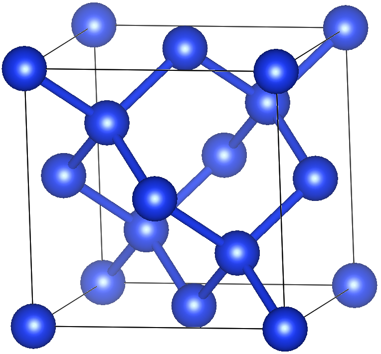
Firsrt run
2025 March 6, updated
Make sure you have the following in your working directory.
- calc_in/
- (cryspy)
- cryspy.in
Then, run CyrSPY!
If you use old version (0.10.3 or earlier):
At the first run, CrySPY goes into structure generation mode.
CrySPY stops after 5 structure generation.
If it worked properly, the following output appears on the screen:
[2025-03-06 18:52:21,495][cryspy_init][INFO]


Start CrySPY 1.4.0b10


[2025-03-06 18:52:21,495][cryspy_init][INFO] # ---------- Library version info
[2025-03-06 18:52:21,495][cryspy_init][INFO] pandas version: 2.2.2
[2025-03-06 18:52:21,495][cryspy_init][INFO] pymatgen version: 2025.1.24
[2025-03-06 18:52:21,495][cryspy_init][INFO] pyxtal version: 1.0.6
[2025-03-06 18:52:21,495][cryspy_init][INFO] # ---------- Read input file, cryspy.in
[2025-03-06 18:52:21,496][write_input][INFO] [basic]
[2025-03-06 18:52:21,496][write_input][INFO] algo = RS
[2025-03-06 18:52:21,496][write_input][INFO] calc_code = ASE
[2025-03-06 18:52:21,496][write_input][INFO] tot_struc = 5
[2025-03-06 18:52:21,496][write_input][INFO] nstage = 1
[2025-03-06 18:52:21,496][write_input][INFO] njob = 2
[2025-03-06 18:52:21,496][write_input][INFO] jobcmd = zsh
[2025-03-06 18:52:21,496][write_input][INFO] jobfile = job_cryspy
...
(omitted)
...
[2025-03-06 18:52:21,497][rs_gen][INFO] # ---------- Initial structure generation
[2025-03-06 18:52:21,497][rs_gen][INFO] # ------ mindist
[2025-03-06 18:52:21,498][struc_util][INFO] Cu - Cu: 1.32
[2025-03-06 18:52:21,498][rs_gen][INFO] # ------ generate structures
[2025-03-06 18:52:21,519][gen_pyxtal][INFO] Structure ID      0: (8,) Space group:  31 -->  31 Pmn2_1
[2025-03-06 18:52:21,525][gen_pyxtal][INFO] Structure ID      1: (8,) Space group: 198 --> 198 P2_13
[2025-03-06 18:52:21,554][gen_pyxtal][INFO] Structure ID      2: (8,) Space group:   4 -->   4 P2_1
[2025-03-06 18:52:21,580][gen_pyxtal][INFO] Structure ID      3: (8,) Space group: 193 --> 191 P6/mmm
[2025-03-06 18:52:21,581][gen_pyxtal][WARNING] Compoisition [8] not compatible with symmetry 172:     spg = 172 retry.
[2025-03-06 18:52:21,625][gen_pyxtal][INFO] Structure ID      4: (8,) Space group:  64 -->  64 Cmce
[2025-03-06 18:52:22,013][cryspy_init][INFO] Elapsed time for structure generation: 0:00:00.516183
Several output files are also generated.
- (
cryspy.out): Short log. only version 0.10.3 or earlier. cryspy.stat: Status file.data/init_POSCARS: Initial struture file in POSCAR format.
You can open this file using VESTAdata/pkl_data: Directory to save pickled data.log_cryspy: log.err_cryspy: error and warning.
Let’s take a look at cryspy.stat file.
[status]
id_queueing = 0 1 2 3 4
Structure ID 0 – 4 are queueing because we just generated structures, and have not submitted yet.
Tip
Check the initial structures, if the distances between atoms are too close, you should set the mindist in cryspy.in.
Submit job
2023 July 10, update
Continue
CrySPY continues the simulation if you have cryspy.stat file.
Tip
Continue if you have crypy.stat
Start from the beginning if you don’t have cryspy.stat
Submit job
Run CyrSPY again.
Check the screen or log_cryspy file.
[2023-07-10 18:52:51,859][cryspy_restart][INFO]


Restart CrySPY 1.2.0


[2023-07-10 18:52:51,869][ctrl_job][INFO] # ---------- job status
[2023-07-10 18:52:51,904][ctrl_job][INFO] ID      0: submit job, Stage 1
[2023-07-10 18:52:51,931][ctrl_job][INFO] ID      1: submit job, Stage 1
And also cryspy.stat file.
...
(omit)
...
[status]
id_queueing = 2 3 4
id      0 = Stage 1
id      1 = Stage 1
CrySPY submitted two jobs for structure ID 0 and 1 as you set njob = 2 in cryspy.in.
Calculations are performed in the work directory.
These directory names correspond to their structure ID.
work
├── 000000
├── 000001
└── fin
When the two jobs are done, run CrySPY again.
[2023-07-10 18:55:01,053][cryspy_restart][INFO]


Restart CrySPY 1.2.0


[2023-07-10 18:55:01,058][ctrl_job][INFO] # ---------- job status
[2023-07-10 18:55:01,058][ctrl_job][INFO] ID      0: Stage 1 Done!
[2023-07-10 18:55:01,093][ctrl_job][INFO]     collect results: E = -0.00696997755502915 eV/atom
[2023-07-10 18:55:01,132][ctrl_job][INFO] ID      1: Stage 1 Done!
[2023-07-10 18:55:01,133][ctrl_job][INFO]     collect results: E = 0.4934076667166454 eV/atom
[2023-07-10 18:55:01,144][cryspy][INFO]

recheck 1

[2023-07-10 18:55:01,145][ctrl_job][INFO] # ---------- job status
[2023-07-10 18:55:01,153][ctrl_job][INFO] ID      2: submit job, Stage 1
[2023-07-10 18:55:01,161][ctrl_job][INFO] ID      3: submit job, Stage 1
If you set nstage = 2 (more than 2), new jobs on stage 2 for ID 0 and 1 are submitted.
If you set nstage = 1, CrySPY collects calculation data of ID 0 and 1, then submits next ID’s jobs.
Directories of the finished structure are moved to the fin directory.
Repeat cryspy several times until all 5 structures are done.
You can delete the work directory when the simulation is done if you do not need it.
The auto script (repeat_cryspy) may help you.
Check results
Move to data directory. There should be a few more files.
$ cd data
$ ls
cryspy_rslt  cryspy_rslt_energy_asc  init_POSCARS  opt_POSCARS  pkl_data/
cryspy_rslt: Result file.cryspy_rslt_energy_asc: Result file sorted in energy ascending order.init_POSCARS: Initial struture file in POSCAR format.opt_POSCARS: Optimized structure file in POSCAR format.pkl_data/: Directory to save pickled data.
The results are written to text files, cryspy_rslt and cryspy_rslt_energy_asc (and also saved in pickle data in pkl_data directory).
Each result appends to cryspy_rslt file in the order in which one finished earlier.
   Spg_num Spg_sym  Spg_num_opt Spg_sym_opt  E_eV_atom  Magmom      Opt
0      139  I4/mmm          139      I4/mmm  -3.000850     NaN     done
1       98  I4_122           12        C2/m  -3.978441     NaN  not_yet
2       16    P222           16        P222  -3.348616     NaN  not_yet
3       36  Cmc2_1           36      Cmc2_1  -3.520306     NaN  not_yet
4       36  Cmc2_1            4        P2_1  -3.304168     NaN  not_yet
Info
Not ID order in cryspy_rslt
In cryspy_rslt_energy_asc file, the results are sorted in energy ascending order.
cat cryspy_rslt_energy_asc
   Spg_num Spg_sym  Spg_num_opt Spg_sym_opt  E_eV_atom  Magmom      Opt
1       98  I4_122           12        C2/m  -3.978441     NaN  not_yet
3       36  Cmc2_1           36      Cmc2_1  -3.520306     NaN  not_yet
2       16    P222           16        P222  -3.348616     NaN  not_yet
4       36  Cmc2_1            4        P2_1  -3.304168     NaN  not_yet
0      139  I4/mmm          139      I4/mmm  -3.000850     NaN     done
Spg_num and Spg_sym show space group information on initial structures.
Spg_num_opt and Spg_sym_opt are those of optimized structures.
The last column Opt indicates whether or not optimization reached required accuracy.
Append structures
Of course only 5 structures are not enough to find stable structures.
You can append structures whenever you want.
Here let’s append more 5 structures.
For Si-Si mindist, the default value of 1.11 Å is used in the first structure generation (see log_cryspy), which is a little too close.
Let us try to set the mindist to 2.0 Å.
Edit cryspy.in and change the value of tot_struc into 10, and add mindist_1 = 2.0
emacs cryspy.in
cat cryspy.in
[basic]
algo = RS
calc_code = soiap
tot_struc = 10
nstage = 1
njob = 2
jobcmd = zsh
jobfile = job_cryspy

[structure]
atype = Si
nat = 8
mindist_1 = 2.0

[soiap]
soiap_infile = soiap.in
soiap_outfile = soiap.out
soiap_cif = initial.cif

[option]
Then run cryspy, and check log_cryspy file.
...
(omit)
...

2023/03/19 00:01:47
CrySPY 1.0.0
Restart cryspy.py


Changed tot_struc from 5 to 10
Changed mindist from None to [[2.0]]

Backup data

# ---------- Append structures
# ------ mindist
Si - Si 2.0
Structure ID      5 was generated. Space group: 218 --> 221 Pm-3m
Structure ID      6 was generated. Space group:  86 --> 129 P4/nmm
Structure ID      7 was generated. Space group: 129 --> 129 P4/nmm
Structure ID      8 was generated. Space group: 191 --> 191 P6/mmm
Structure ID      9 was generated. Space group:  31 -->  31 Pmn2_1
Remember that CrySPY goes into structure generation mode whenever you change the value of tot_struc.
In this mode, CrySPY does not do any other action such as collecting data, submitting jobs, and so on.
Note
Structure generation mode whenever you change the value of tot_struc.
From version 1.0.0, CrySPY automatically backs up when adding structures.
See features/backup.
Repeat cryspy & several times until all appended structures are done.
The auto script (repeat_cryspy) may help you.
Analysis and visualization
Download data
It is assumed here that you analyze and visualize CrySPY data on your local PC.
If you use CrySPY on a supercomputer or workstation, download the data to your local machine.
You can delete the work and backup directories if they are not needed, as their file size can be very large.
Jupyter notebook
Move to the data/ directory in the results you downloaded earlier.
Then, if the CrySPY utility has already been downloaded locally, copy cryspy_analyzer_RS.ipynb.
Alternatively, you can download it directly from GitHub (CrySPY_utility/notebook/).
Launch Jupyter (e.g., VS Code, Jupyter Lab, or Jupyter Notebook),
and simply run the cells in order to obtain a figure like the one shown below.

Subsections of Variable-composition evolutionary algorithm (EA-vc)
ASE on your local PC (Cu-Ag-Au)
2025 July 11, updated
The files used in this tutorial can be downloaded from CrySPY_utility/examples/ase_Cu-Ag-Au_EA-vc.
This tutorial demonstrates a test run on a local machine using ASE’s lightweight Pure Python EMT calculator.
The target system is the ternary Cu-Ag-Au system.
cryspy.in
Example of cryspy.in.
[basic]
algo = EA-vc
calc_code = ASE
nstage = 1
njob = 5
jobcmd = zsh
jobfile = job_cryspy
[structure]
atype = Cu Ag Au
ll_nat = 0 0 0
ul_nat = 8 8 8
[ASE]
ase_python = ase_in.py
[EA]
n_pop = 20
n_crsov = 5
n_perm = 2
n_strain = 2
n_rand = 2
n_add = 3
n_elim = 3
n_subs = 3
target = random
n_elite = 2
n_fittest = 10
slct_func = TNM
t_size = 2
end_point = 0.0 0.0 0.0
maxgen_ea = 0
[option]
calc_in/
The contents under calc_in/ are the same as those in Tutorial > Random Search (RS) > ASE on your local PC.
calc_in/ase_in.py
from ase.constraints import FixSymmetry
from ase.filters import FrechetCellFilter
from ase.calculators.emt import EMT
from ase.optimize import BFGS
import numpy as np
from ase.io import read, write
# ---------- input structure
# CrySPY outputs 'POSCAR' as an input file in work/xxxxxx directory
atoms = read('POSCAR', format='vasp')
# ---------- setting and run
atoms.calc = EMT()
atoms.set_constraint([FixSymmetry(atoms)])
cell_filter = FrechetCellFilter(atoms, hydrostatic_strain=False)
opt = BFGS(cell_filter)
# ---------- run
converged = opt.run(fmax=0.01, steps=2000)
# ---------- rule in ASE interface
# output file for energy: 'log.tote' in eV/cell
# CrySPY reads the last line of 'log.tote' file
# outimized structure: 'CONTCAR' file in vasp format
# check_opt: 'out_check_opt' file ('done' or 'not yet')
# CrySPY reads the last line of 'out_check_opt' file
# ------ energy
e = cell_filter.atoms.get_total_energy() # eV/cell
with open('log.tote', mode='w') as f:
f.write(str(e))
# ------ struc
opt_atoms = cell_filter.atoms.copy()
opt_atoms.set_constraint(None) # remove constraint for pymatgen
write('CONTCAR', opt_atoms, format='vasp', direct=True)
# ------ check_opt
with open('out_check_opt', mode='w') as f:
if converged:
f.write('done\n')
else:
f.write('not yet\n')
calc_in/job_cryspy
#!/bin/sh

# ---------- ASE
python3 ase_in.py > out.log
ASE-CHGNet(Cu-Au)
2025 July 11, updated
Info
CHGNet needs to be installed.
The files used in this tutorial can be downloaded from CrySPY_utility/examples/ase_chgnet_Cu-Au_EA-vc.
In this tutorial, we assume that a computing cluster with a job scheduler is used together with the machine learning potential CHGNet.
The calculation can also be performed on a local PC, so if you prefer this, please modify the input settings accordingly.
The target system is the binary Cu-Au system.
Pre-calculation
In EA-vc, the per-atom energies of each elemental phase must be used as the reference in the end_point setting of cryspy.in, so they need to be calculated beforehand.
There should be two directories inside the example.
Au_fcc
├── POSCAR
├── chgnet_in.py
└── job_cryspy
Cu_fcc
├── POSCAR
├── chgnet_in.py
└── job_cryspy
Each directory contains a crystal structure file (POSCAR), a Python script (chgnet_in.py) to perform structure relaxation and calculate energy, and a job script (job_cryspy).
Please modify these files according to your computing environment.
Submit the job (replace the job submission command as appropriate for your system).
cd Au_fcc
qsub job_cryspy
cd ../Cu_fcc
qsub job_cryspy
cd ..
When the calculations finish successfully, a file named end_point will be created in each directory, containing the energy per atom (eV/atom) after structure relaxation.
cat Au_fcc/end_point
-3.2357187271118164
cat Cu_fcc/end_point
-4.083529472351074
These values are then used as input for the cryspy.in file.
cryspy.in
[basic]
algo = EA-vc
calc_code = ASE
nstage = 1
njob = 20
jobcmd = qsub
jobfile = job_cryspy
[structure]
atype = Cu Au
ll_nat = 0 0
ul_nat = 8 8
[ASE]
ase_python = chgnet_in.py
[EA]
n_pop = 20
n_crsov = 5
n_perm = 2
n_strain = 2
n_rand = 2
n_add = 3
n_elim = 3
n_subs = 3
target = random
n_elite = 2
n_fittest = 10
slct_func = TNM
t_size = 2
maxgen_ea = 0
end_point = -4.08352709 -3.23571777
[option]
calc_in/
The contents under calc_in/ are the same as those in Tutorial > Random Search (RS) > ASE on your local PC, with minor modifications for CHGNet.
Be sure to adjust paths such as the Python executable in the job script to match your computing environment.
Be sure to adjust the Python executable path in the job script.
calc_in/chgnet_in.py
# ---------- import
from ase.constraints import FixSymmetry
from ase.filters import FrechetCellFilter
from ase.io import read, write
from ase.optimize import FIRE, BFGS, LBFGS
from chgnet.model import CHGNetCalculator
# ---------- input structure
# CrySPY outputs 'POSCAR' as an input file in work/xxxxxx directory
atoms = read('POSCAR')
# ---------- set up
atoms.calc = CHGNetCalculator()
atoms.set_constraint([FixSymmetry(atoms)])
cell_filter = FrechetCellFilter(atoms)
opt = BFGS(cell_filter, trajectory='opt.traj')
# ---------- run
converged = opt.run(fmax=0.01, steps=2000)
# ---------- rule in ASE interface
# output file for energy: 'log.tote' in eV/cell
# CrySPY reads the last line of 'log.tote' file
# outimized structure: 'CONTCAR' file in vasp format
# check_opt: 'out_check_opt' file ('done' or 'not yet')
# CrySPY reads the last line of 'out_check_opt' file
# ------ energy
e = cell_filter.atoms.get_total_energy() # eV/cell
with open('log.tote', mode='w') as f:
f.write(str(e))
# ------ struc
opt_atoms = cell_filter.atoms.copy()
opt_atoms.set_constraint(None) # remove constraint for pymatgen
write('CONTCAR', opt_atoms, format='vasp', direct=True)
# ------ check_opt
with open('out_check_opt', mode='w') as f:
if converged:
f.write('done\n')
else:
f.write('not yet\n')
calc_in/job_cryspy
#!/bin/sh
#$ -cwd
#$ -V -S /bin/bash
####$ -V -S /bin/zsh
#$ -N CuAu_CrySPY_ID
#$ -pe smp 2
# ---------- OpenMP
export OMP_NUM_THREADS=2
# ---------- ASE
/usr/local/Python-3.10.13/bin/python3 chgnet_in.py > out.log
VASP(Fe-Al)
2025 July 12
EA-vc became compatible with VASP in version 1.4.2.
The files used here can be downloaded from CrySPY_utility/examples/vasp_Fe-Al_EA-vc.
This tutorial assumes calculations are performed on a computer cluster with a job scheduler using VASP.
The target system is a binary Fe-Al alloy, and calculations are performed assuming ferromagnetism.
Pre-calculation
In EA-vc, the per-atom energies of each elemental phase must be used as the reference in the end_point setting of cryspy.in, so they need to be calculated beforehand.
There should be two directories inside the example.
Al-fcc
├── POSCAR
├── INCAR
├── POTCAR_dummy
└── job_cryspy
Fe-bcc
├── POSCAR
├── INCAR
├── POTCAR_dummy
└── job_cryspy
Crystal structure data (POSCAR), input files for structure optimization and energy calculation (INCAR), and job scripts (job_cryspy) are provided, so edit them as needed to match your computing environment.
Also, the POTCAR files cannot be distributed, so please prepare them yourself.
In the INCAR file, be sure to use the same cutoff and other values for the single-element calculations as you will use in the final calculations.
Run the jobs (replace the job submission command as appropriate for your environment).
cd Al_fcc
qsub job_cryspy
cd ../Fe_bcc
qsub job_cryspy
cd ..
After the calculations are finished, obtain the energy per atom.
In this case, since BCC and FCC unit cells each contain one atom, you can use the total energy value directly.
Normally, divide the total energy by the number of atoms in the unit cell to obtain the per-atom energy.
cryspy.in
cryspy.in
[basic]
algo = EA-vc
calc_code = VASP
nstage = 2
njob = 10
jobcmd = qsub
jobfile = job_cryspy
[structure]
atype = Fe Al
ll_nat = 0 0
ul_nat = 8 8
[VASP]
kppvol = 40 120
vasp_MAGMOM = 4.0 0.0
[EA]
n_pop = 20
n_crsov = 5
n_perm = 2
n_strain = 2
n_rand = 2
n_add = 3
n_elim = 3
n_subs = 3
target = random
n_elite = 2
n_fittest = 10
slct_func = TNM
t_size = 2
maxgen_ea = 0
end_point = -8.24249611 -3.74226843
[option]
for VASP
In the [VASP] section, specify the MAGMOM values for each element corresponding to atype in vasp_MAGMOM.
When CrySPY copies the INCAR file to ./work/xxx/INCAR (where xxx is the structure ID), it appends n*vasp_MAGMOM (n is the number of atoms).
For example, if atype = (‘Fe’, ‘Al’), nat = (5, 3), and vasp_MAGMOM = (4.0 0.0), the following will be appended.
Although not used in this tutorial, INCAR’s LDAUL, LDAUU, and LDAUJ are also supported. In cryspy.in, they are used with the vasp_ prefix as follows:
[VASP]
kppvol = 40 120
vasp_MAGMOM = 4.0 0.0
vasp_LDAUL = 2 -1
vasp_LDAUU = 4.0 0.0
vasp_LDAUJ = 0.0 0.0
If the system changes from a binary alloy to a single element, such as nat = (5, 0), CrySPY will append the following to ./work/xxx/INCAR.
No action is taken for elements with an atomic number of zero.
MAGMOM = 5*4.0
LDAUL = 2
LDAUU = 4.0
LDAUJ = 0.0
calc_in/
POTCAR
In EA-vc, prepare a separate POTCAR file for each element.
The file names should be:
Add the element name as written in atype to the end of the file name.
CrySPY prepares ./work/xxx/POTCAR according to the number of atoms in the structure.
For example, if the structure consists only of Fe (nat = (5, 0)), use POTCAR_Fe.
If the structure is Fe-Al (nat = (4, 4)), concatenate POTCAR_Fe and POTCAR_Al to create POTCAR.
job_cryspy
#!/bin/sh
#$ -cwd
#$ -V -S /bin/bash
####$ -V -S /bin/zsh
#$ -N FeAl_CrySPY_ID
#$ -pe smp 32
# ---------- vasp
VASPROOT=/usr/local/vasp/vasp.6.4.2/bin
mpirun -np $NSLOTS $VASPROOT/vasp_std
INCAR
1_INCAR
SYSTEM = FeAl
Algo = Fast
####LREAL = Auto
ENCUT = 348
ISMEAR = 1
SIGMA = 0.1
NSW = 40
IBRION = 2
ISIF = 2
ISPIN = 2
######MAGMOM = # cryspy append MAGMOM in work/xx/INCAR
EDIFF = 1e-6
EDIFFG = -0.01
KPAR = 4
LWAVE = .FALSE.
LCHARG = .FALSE.
2_INCAR
SYSTEM = FeAl
Algo = Fast
####LREAL = Auto
ENCUT = 348
ISMEAR = 1
SIGMA = 0.1
NSW = 200
IBRION = 2
ISIF = 3
ISPIN = 2
######MAGMOM = # cryspy append MAGMOM in work/xx/INCAR
EDIFF = 1e-6
EDIFFG = -0.01
KPAR = 4
LWAVE = .FALSE.
LCHARG = .FALSE.
QE(Fe-Al)
2025 July 18
EA-vc became compatible with QE in version 1.4.2.
The files used here can be downloaded from CrySPY_utility/examples/qe_Fe-Al_EA-vc.
This tutorial assumes calculations are performed on a computer cluster with a job scheduler using QE.
The target system is a binary Fe-Al alloy, and calculations are performed assuming ferromagnetism.
Pre-calculation
In EA-vc, the per-atom energies of each elemental phase must be used as the reference in the end_point setting of cryspy.in, so they need to be calculated beforehand.
There should be two directories inside the example.
Al-fcc
├── pwscf.in
└── job_cryspy
Fe-bcc
├── pwscf.in
└── job_cryspy
Input files (pwscf.in) and job scripts (job_cryspy) are provided, so edit them as needed to match your computing environment.
In the pwscf.in file, be sure to use the same cutoff and other values for the single-element calculations as you will use in the final calculations.
Run the jobs (replace the job submission command as appropriate for your environment).
cd Al_fcc
qsub job_cryspy
cd ../Fe_bcc
qsub job_cryspy
cd ..
After the calculations are finished, convert the energy per atom to eV units.
In this case, since BCC and FCC unit cells each contain one atom, you can use the total energy value directly.
Normally, divide the total energy by the number of atoms in the unit cell to obtain the per-atom energy.
cryspy.in
cryspy.in
[basic]
algo = EA-vc
calc_code = QE
nstage = 2
njob = 10
jobcmd = qsub
jobfile = job_cryspy
[structure]
atype = Fe Al
ll_nat = 0 0
ul_nat = 8 8
[QE]
kppvol = 40 120
qe_infile = pwscf.in
qe_outfile = pwscf.out
[EA]
n_pop = 20
n_crsov = 5
n_perm = 2
n_strain = 2
n_rand = 2
n_add = 3
n_elim = 3
n_subs = 3
target = random
n_elite = 2
n_fittest = 10
slct_func = TNM
t_size = 2
maxgen_ea = 6
end_point = -3406.14117375 -91.25463006
[option]
for QE
Unlike VASP, support for variable-composition in QE is straightforward.
For binary system searches, always prepare binary system inputs in ./calc_in, and for ternary systems, always prepare ternary system inputs.
However, only nat needs to be changed, so CrySPY automatically rewrites it.
When preparing, write nat with any appropriate number as shown below:
In ./work/xxx/, CrySPY automatically rewrites lines that start with nat (excluding leading whitespace) to:
nat = (actual number of atoms)
calc_in/
job_cryspy
#!/bin/sh
#$ -cwd
#$ -V -S /bin/bash
####$ -V -S /bin/zsh
#$ -N FeAl_CrySPY_ID
#$ -pe smp 32
QEROOT=/usr/local/qe/q-e-qe-7.3.1/bin
mpirun -np $NSLOTS $QEROOT/pw.x -nk 4 < pwscf.in > pwscf.out
if [ -e "CRASH" ]; then
sed -i -e '3 s/^.*$/skip/' stat_job
exit 1
fi
pwscf.in
1_pwscf.in
&control
calculation = 'relax'
nstep = 40
pseudo_dir = '/usr/local/qe/gbrv/all_pbe_UPF_v1.5/'
outdir='./outdir/'
/
&system
ibrav = 0
nat = 1
ntyp = 2
ecutwfc = 40
ecutrho = 200
occupations = "smearing"
smearing = "mp"
degauss = 0.01
nspin = 2
starting_magnetization(1) = 0.4
starting_magnetization(2) = 0.0
/
&electrons
mixing_beta = 0.4
/
&ions
/
&cell
/
ATOMIC_SPECIES
Fe -1.0 fe_pbe_v1.5.uspp.F.UPF
Al -1.0 al_pbe_v1.uspp.F.UPF
2_pwscf.in
&control
calculation = 'vc-relax'
nstep = 200
pseudo_dir = '/usr/local/qe/gbrv/all_pbe_UPF_v1.5/'
outdir='./outdir/'
/
&system
ibrav = 0
nat = 1
ntyp = 2
ecutwfc = 40
ecutrho = 200
occupations = "smearing"
smearing = "mp"
degauss = 0.01
nspin = 2
starting_magnetization(1) = 0.4
starting_magnetization(2) = 0.0
/
&electrons
mixing_beta = 0.4
/
&ions
/
&cell
/
ATOMIC_SPECIES
Fe -1.0 fe_pbe_v1.5.uspp.F.UPF
Al -1.0 al_pbe_v1.uspp.F.UPF
Create next generation
2025 June 16
First run
When you run cryspy, the program enters structure generation mode.
It generates the first generation of random structures and then exits.
It can be confirmed from the output that structures are generated with the number of atoms within the range specified by ll_nat and ul_nat.
...
[2025-06-16 10:04:45,648][cryspy_init][INFO] # ---------- Initial structure generation
[2025-06-16 10:04:45,648][rs_gen][INFO] # ------ mindist
[2025-06-16 10:04:45,650][struc_util][INFO] Cu - Cu: 1.32
[2025-06-16 10:04:45,650][struc_util][INFO] Cu - Ag: 1.385
[2025-06-16 10:04:45,650][struc_util][INFO] Cu - Au: 1.34
[2025-06-16 10:04:45,650][struc_util][INFO] Ag - Ag: 1.45
[2025-06-16 10:04:45,650][struc_util][INFO] Ag - Au: 1.405
[2025-06-16 10:04:45,650][struc_util][INFO] Au - Au: 1.36
[2025-06-16 10:04:45,650][rs_gen][INFO] # ------ generate structures
[2025-06-16 10:04:45,659][gen_pyxtal][WARNING] Compoisition [1 4] not compatible with symmetry 34: spg = 34 retry.
[2025-06-16 10:04:45,662][gen_pyxtal][WARNING] Compoisition [ 2 2 12] not compatible with symmetry 39: spg = 39 retry.
[2025-06-16 10:04:45,691][gen_pyxtal][INFO] Structure ID 0: (3, 1, 2) Space group: 82 --> 119 I-4m2
[2025-06-16 10:04:45,694][gen_pyxtal][WARNING] Compoisition [6 6 2] not compatible with symmetry 57: spg = 57 retry.
[2025-06-16 10:04:45,749][gen_pyxtal][INFO] Structure ID 1: (1, 8, 5) Space group: 71 --> 71 Immm
[2025-06-16 10:04:45,857][gen_pyxtal][INFO] Structure ID 2: (3, 7, 8) Space group: 174 --> 174 P-6
...
The file cryspy.stat shows that the current generation’s information is being added during the EA process.
[status]
generation = 1
id_queueing = 0 1 2 3 4 5 6 7 8 9 10 11 12 13 14 15 16 17 18 19
Optimize structures
After running cryspy several times and completing the structure optimization for the first generation, the output will appear as shown below.
...
[2025-06-16 10:25:56,962][ctrl_job][INFO] Done generation 1
[2025-06-16 10:25:56,962][ctrl_job][INFO] Calculate convex hull for generation 1
[2025-06-16 10:25:57,854][ctrl_job][INFO]
EA is ready
Convex hull
At this point, the hull distance data and the convex hull plot have been output to ./data/convex_hull/.
    ID    hull distance (eV/atom)    Num_atom
     7                   0.000000    (0, 2, 6)
    14                   0.036510    (1, 7, 6)
    17                   0.064702    (0, 1, 5)
    19                   0.113649    (0, 0, 8)
    16                   0.168530    (6, 4, 8)
     9                   0.186497    (8, 4, 6)
     1                   0.187379    (1, 8, 5)
    11                   0.233893    (4, 5, 4)
     3                   0.273365    (6, 5, 5)
    10                   0.326759    (1, 4, 4)
     2                   0.330749    (3, 7, 8)
     8                   0.359543    (6, 2, 7)
     4                   0.404169    (4, 4, 2)
    18                   0.422989    (0, 6, 8)
    13                   0.428456    (0, 6, 3)
     5                   0.444792    (7, 4, 7)
     6                   0.464305    (7, 7, 7)
    12                   0.556654    (3, 0, 0)
    15                   0.560062    (6, 7, 1)
     0                   0.644278    (3, 1, 2)
- conv_hull_gen_1.svg

Create next generation
Once all preparations are complete, running cryspy again automatically creates a backup and starts generating the next-generation structures.
...
[2025-06-16 10:37:19,860][ctrl_job][INFO] Done generation 1
[2025-06-16 10:37:20,136][utility][INFO] Backup data
[2025-06-16 10:37:20,173][ea_next_gen][INFO] # ---------- Evolutionary algorithm
[2025-06-16 10:37:20,174][ea_next_gen][INFO] Generation 2
[2025-06-16 10:37:20,174][ea_next_gen][INFO] # ------ natural selection
[2025-06-16 10:37:20,177][ea_next_gen][INFO] ranking without duplication (including elite):
[2025-06-16 10:37:20,177][ea_next_gen][INFO] Structure ID      7, fitness:    0.00000
[2025-06-16 10:37:20,177][ea_next_gen][INFO] Structure ID     14, fitness:    0.03651
[2025-06-16 10:37:20,177][ea_next_gen][INFO] Structure ID     17, fitness:    0.06470
[2025-06-16 10:37:20,177][ea_next_gen][INFO] Structure ID     19, fitness:    0.11365
[2025-06-16 10:37:20,177][ea_next_gen][INFO] Structure ID     16, fitness:    0.16853
[2025-06-16 10:37:20,177][ea_next_gen][INFO] Structure ID      9, fitness:    0.18650
[2025-06-16 10:37:20,177][ea_next_gen][INFO] Structure ID      1, fitness:    0.18738
[2025-06-16 10:37:20,177][ea_next_gen][INFO] Structure ID     11, fitness:    0.23389
[2025-06-16 10:37:20,177][ea_next_gen][INFO] Structure ID      3, fitness:    0.27336
[2025-06-16 10:37:20,177][ea_next_gen][INFO] Structure ID     10, fitness:    0.32676
[2025-06-16 10:37:20,177][ea_next_gen][INFO] # ------ Generate children
[2025-06-16 10:37:20,177][ea_child][INFO] # -- mindist
[2025-06-16 10:37:20,179][struc_util][INFO] Cu - Cu: 1.32
[2025-06-16 10:37:20,179][struc_util][INFO] Cu - Ag: 1.385
[2025-06-16 10:37:20,179][struc_util][INFO] Cu - Au: 1.34
[2025-06-16 10:37:20,179][struc_util][INFO] Ag - Ag: 1.45
[2025-06-16 10:37:20,179][struc_util][INFO] Ag - Au: 1.405
[2025-06-16 10:37:20,179][struc_util][INFO] Au - Au: 1.36
[2025-06-16 10:37:20,217][crossover][INFO] Structure ID     20 (0, 4, 7) was generated from     19 and     14 by crossover. Space group:   1 P1
[2025-06-16 10:37:20,219][crossover][INFO] Structure ID     21 (0, 1, 7) was generated from      7 and     17 by crossover. Space group:   1 P1
[2025-06-16 10:37:20,221][crossover][INFO] Structure ID     22 (3, 0, 8) was generated from     16 and     19 by crossover. Space group:   1 P1
[2025-06-16 10:37:20,225][crossover][INFO] Structure ID     23 (0, 1, 7) was generated from      7 and     17 by crossover. Space group:   1 P1
...
[2025-06-16 10:37:20,809][ea_next_gen][INFO] # ------ Select elites
[2025-06-16 10:37:20,809][ea_next_gen][INFO] Structure ID      7 keeps as the elite
[2025-06-16 10:37:20,809][ea_next_gen][INFO] Structure ID     14 keeps as the elite
After that, simply running cryspy repeatedly will advance the structure search.
Check results
This section focuses on the differences from the EA method.
cryspy_rslt
Below is an example of a cryspy_rslt file after completing calculations up to the third generation.
In EA-vc, formation energy (Ef_eV_atom) and number of atoms (Num_atom) are also included.
    Gen  Spg_num Spg_sym  Spg_num_opt Spg_sym_opt  E_eV_atom  Ef_eV_atom   Num_atom  Magmom      Opt
0     1      119   I-4m2          119       I-4m2   0.639865    0.639865  (3, 1, 2)     NaN  no_file
1     1       71    Immm           71        Immm   0.182650    0.182650  (1, 8, 5)     NaN  no_file
2     1      174     P-6          187       P-6m2   0.324864    0.324864  (3, 7, 8)     NaN  no_file
3     1       71    Immm           71        Immm   0.269227    0.269227  (6, 5, 5)     NaN  no_file
4     1       12    C2/m           65        Cmmm   0.401521    0.401521  (4, 4, 2)     NaN  no_file
7     1      123  P4/mmm          123      P4/mmm  -0.009930   -0.009930  (0, 2, 6)     NaN  no_file
10    1      107    I4mm          107        I4mm   0.320875    0.320875  (1, 4, 4)     NaN  no_file
5     1      121   I-42m          121       I-42m   0.439643    0.439643  (7, 4, 7)     NaN  no_file
6     1      115   P-4m2          115       P-4m2   0.459892    0.459892  (7, 7, 7)     NaN  no_file
8     1       81     P-4           81         P-4   0.354247    0.354247  (6, 2, 7)     NaN  no_file
9     1       11  P2_1/m           11      P2_1/m   0.182084    0.182084  (8, 4, 6)     NaN  no_file
11    1       10    P2/m           10        P2/m   0.229819    0.229819  (4, 5, 4)     NaN  no_file
nat_data
Information on the number of atoms is also included in nat_data.
    ID    ('Cu', 'Ag', 'Au')
     0    (3, 1, 2)
     1    (1, 8, 5)
     2    (3, 7, 8)
     3    (6, 5, 5)
     4    (4, 4, 2)
     5    (7, 4, 7)
     6    (7, 7, 7)
     7    (0, 2, 6)
     8    (6, 2, 7)
     9    (8, 4, 6)
    10    (1, 4, 4)
...
hull_dist_all_gen_x
For example, after the third generation is completed, the hull distance data is output to the file ./convex_hull/hull_dist_all_gen_3.
    ID    hull distance (eV/atom)    Num_atom
    43                   0.000000    (0, 2, 5)
    42                   0.000000    (0, 5, 5)
    48                   0.000000    (0, 1, 5)
    46                   0.000009    (0, 1, 5)
    28                   0.000011    (0, 1, 5)
    41                   0.000360    (0, 4, 6)
    47                   0.001838    (0, 1, 5)
    36                   0.001992    (1, 1, 6)
    21                   0.002544    (0, 1, 7)
    23                   0.002551    (0, 1, 7)
    24                   0.002795    (0, 4, 7)
conv_hull_gen_x.svg
The convex hull plot at the end of generation 3 is saved as ./convex_hull/conv_hull_gen_3.svg.
Although svg is the default format, it can be changed to pdf or png by modifying the fig_format in the input file.

Analysis and visualization
Automatic convex hull plotting
In EA-vc simulations of binary and ternary systems, a convex hull plot is automatically generated at the end of each generation.
For further customization, you can edit the plot yourself using a Jupyter notebook.
For quaternary systems, visualization using Plotly with Jupyter is available (Plotly should already be installed automatically, as it is a dependency of pymatgen).
Below are some usage examples.
Binary system

The above figure shows an example after search up to the third generation, with red labels added for explanation.
The input file settings related to convex hull plotting are listed below (default values in parentheses).
show_max: Upper limit of the y-axis (0.2)label_stable: Whether to display compositions of stable phases (True)vmax: Maximum value of the colorbar on the right (0.2)bottom_margin: Margin between the minimum value and the lower end of the y-axis (0.02)fig_format: File format of the output figure. Supported formats: svg, png, pdf. (svg)
Each marker corresponding to the latest generation is marked with a cross.
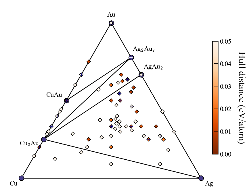
Ternary system

The above figure shows an example after search up to the third generation, with red labels added for explanation.
The input file settings related to convex hull plotting are listed below (default values in parentheses).
show_max: Only entries with a hull distance less than or equal to show_max are plotted. (0.2)label_stable: Whether to display compositions of stable phases (True)vmax: Maximum value of the colorbar on the right (0.2)bottom_margin: Not applicable to ternary systemsfig_format: File format of the output figure. Supported formats: svg, png, pdf. (svg)
Each marker corresponding to the latest generation is marked with a cross.
Download data
It is assumed here that you analyze and visualize CrySPY data on your local PC.
If you use CrySPY on a supercomputer or workstation, download the data to your local machine.
You can delete the work and backup directories if they are not needed, as their file size can be very large.
Jupyter notebook
Move to the data/ directory in the results you downloaded earlier.
Then, if the CrySPY utility has already been downloaded locally, copy cryspy_analyzer_EA-vc.ipynb.
Alternatively, you can download it directly from GitHub (CrySPY_utility/notebook/).
The Jupyter notebook file includes the same functions as the CrySPY code, allowing you to freely customize the convex hull plots.
Execute the cells in order as appropriate, and choosing one of the following options will produce the same plot as the automatic output.
- Binary system, matplotlib
- Ternary system, matplotlib
In the section
- Interactive plot using Plotly,
interactive plots using Plotly are available for binary, ternary, and quaternary systems.
See CrySPY > Tutorial > Interactive Mode (Jupyter Notebook) #Interactive plot using Plotly for example plots.
LAQA
May 15th, 2023
The example files used here can be downloaded from CrySPY_utility/examples/qe_Si16_LAQA.
In this tutorial, only 50 initial structures are generated, but originally, LAQA is designed to select candidates from many more structures.
cryspy.in
Here is an example of cryspy.in.
[basic]
algo = LAQA
calc_code = QE
tot_struc = 50
nstage = 1
njob = 10
jobcmd = qsub
jobfile = job_cryspy

[structure]
atype = Si
nat = 16
mindist_1 = 1.5

[QE]
qe_infile = pwscf.in
qe_outfile = pwscf.out
kppvol =  80

[LAQA]
nselect_laqa = 4

[option]
nstage must be 1 in LAQA- You have to write
nselect_laqa in [LAQA] section. nselect_laqa is the number of candidates you select at one time.
If you want to change the value of the weight for LAQA score, edit wf and ws as below.
If omitted, the default values are used (0.1 and 10.0, respectively).
See, Search algorithms > LAQA for the score.
[LAQA]
nselect_laqa = 4
wf = 0.1
ws = 10.0
calc_in/pwscf.in_1
&control
    calculation = 'vc-relax'
    pseudo_dir = '/usr/local/gbrv/all_pbe_UPF_v1.5/'
    outdir='./outdir/'
    nstep = 10
/

&system
    ibrav = 0
    nat = 16
    ntyp = 1
    ecutwfc = 40
    ecutrho = 200
    occupations = 'smearing'
    degauss = 0.01
/

&electrons
/

&ions
/

&cell
/

ATOMIC_SPECIES
  Si -1.0 si_pbe_v1.uspp.F.UPF
nstep controls how many steps of structure optimization can proceed in one selection. (NSW for VASP)
calc_in/job_cryspy
#!/bin/sh
#$ -cwd
#$ -V -S /bin/bash
####$ -V -S /bin/zsh
#$ -N Si_CrySPY_ID
#$ -pe smp 20
####$ -q ibis1.q
####$ -q ibis2.q

mpirun -np $NSLOTS pw.x -nk 4 < pwscf.in > pwscf.out

if [ -e "CRASH" ]; then
    sed -i -e '3 s/^.*$/skip/' stat_job
    exit 1
fi

sed -i -e '3 s/^.*$/done/' stat_job
- The job file is the same as the usual way.
Run
Tip
An automatic script is also available. See the bottom of this page.
Just type cryspy for the 1st run.
cryspy &
Check log_cryspy.
50 random structures are generated.
2023/05/13 13:02:07
CrySPY 1.1.0
Start cryspy.py
Number of MPI processes: 1

Read input file, cryspy.in
Save input data in cryspy.stat

# --------- Generate initial structures
# ------ mindist
Si - Si 1.5
Structure ID      0 was generated. Space group: 165 --> 165 P-3c1
Structure ID      1 was generated. Space group:  66 -->  66 Cccm
Structure ID      2 was generated. Space group: 146 --> 146 R3
Structure ID      3 was generated. Space group:  82 -->  82 I-4
Structure ID      4 was generated. Space group: 162 --> 162 P-31m
...
...
...
Structure ID     47 was generated. Space group:  90 -->  90 P42_12
Structure ID     48 was generated. Space group: 214 --> 214 I4_132
Structure ID     49 was generated. Space group:  23 -->  23 I222

Elapsed time for structure generation: 0:00:10.929030


# ---------- Initialize LAQA
# ---------- Selection 0
selected_id: 50 IDs
In LAQA, jobs of structure optimization for all structures are submitted once at the beginning.
Note that only 10 steps are proceeded here since we set nstep = 10.
Repeat cryspy command until all of these (10 steps) are completed.
If necessary, you can also submit all jobs at once by increasing the value of njob.
After all the initial optimizations, LAQA is ready is displayed at the end of log_cryspy.
2023/05/13 13:23:31
CrySPY 1.1.0
Restart cryspy.py
Number of MPI processes: 1


# ---------- job status
ID     41: Stage 1 Done!

LAQA is ready
Next cryspy run will make the first selection.
2023/05/13 13:23:33
CrySPY 1.1.0
Restart cryspy.py
Number of MPI processes: 1


# ---------- job status

Backup data

# ---------- Selection 1
selected_id: 37 8 10 48
Here, only the number set in nselect_laqa will be selected.
Type cryspy to submit the jobs (next 10 steps).
cryspy &
2023/05/13 13:23:36
CrySPY 1.1.0
Restart cryspy.py
Number of MPI processes: 1


# ---------- job status
ID     37: submit job, Stage 1
ID      8: submit job, Stage 1
ID     10: submit job, Stage 1
ID     48: submit job, Stage 1
Then, by repeating this over and over again, the optimization of the structure selected according to the score advances by 10 steps each time.
Proceed until several structures are completed, and finish (stop) when you like.
Status
If you want to check the LAQA score during the simulation, you can look at the status file:
Other files for LAQA will be output:
- ./data_LAQA_bias
- ./data_LAQA_energy
- ./data_LAQA_score
- ./data_LAQA_selected_id
- ./data_LAQA_step
Analysis and visualization
It is assumed here that you analyze and visualize CrySPY data in your local PC.
If you use CrySPY in super computers or workstations, download the data in your local PC.
You can delete the work and backup directory if you do not need it because the file size could be very large.
You may gzip the pkl data to decrease the file size.
jupyter notebook
Move to the data/ directory in results you just downloaded.
Then copy cryspy_analyzer_LAQA.ipynb from CrySPY utility.
You can obtain the graph and animation with the notebook.
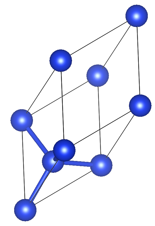
In the gif below, all of the optimizations were completed. This is just for animation.
(When all of the optimizations are completed, the computational cost is the same as random search.)
This graph shows the energy as a function of optimization step.
The red lines indicate three structures with the lowest energy.
The most stable one reached diamond structure.
The structures that eventually become stable were selected at an early stage.
Info
If algo = LAQA, the followings are automatically set in the [option] section.
- force_step_flag = True
- stress_step_flag = True
Force and stress data are collected step by step.
Energy and structure data are NOT. They are collected for each selection.
In other words, in this case, energy and structure data are saved once every 10 steps.
If you want to collect energy and structure data step by step, manually set up as follows:
[option]
energy_step_flag = True
struc_step_flag = True
Auto script
You may find it tedious to run cryspy over and over again.
The auto script could help you.
repeat_cryspy
Molecular crystal structure prediction
In this section, we give a tutorial on the molecular structure generation part only.
Since version 0.9.0, CrySPY has been able to generate random molecular crystal structures using PyXtal.
You need to use a pre-defined molecular by PyXtal’s database (see, https://pyxtal.readthedocs.io/en/latest/Usage.html?highlight=benzene#pyxtal-molecule-pyxtal-molecule))
or create molecule files that define molecular structures.
Pre-defined molecule
PyXtal currently supports C60, H2O, CH4, NH3, benzene, naphthalene, anthracene, tetracene, pentacene, coumarin, resorcinol, benzamide, aspirin, ddt, lindane, glycine, glucose, and ROY.
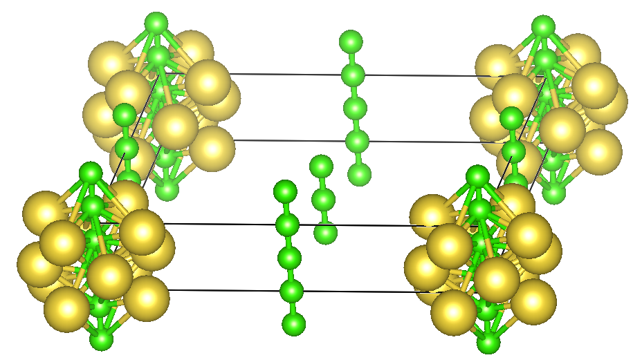
Let us generate molecular crystal structures that consist of 2 benzenes.
Move to your working directory, and copy input example files by one of the following methods.
Take a look at cryspy.in.
$ cat cryspy.in
[basic]
algo = RS
calc_code = QE
tot_struc = 6
nstage = 2
njob = 2
jobcmd = qsub
jobfile = job_cryspy

[structure]
struc_mode = mol
atype = H C
nat = 12 12
mol_file = benzene
nmol = 2

[QE]
qe_infile = pwscf.in
qe_outfile = pwscf.out
kppvol = 40  60

[option]
In generating molecular crystal structures, you have to set struc_mode = mol in the [structure] section.
Molecule file(s) and the number of molecule(s) are specified as:
- mol_file = benzene
- nmol = 2
Run CrySPY and see the initial structures (./data/init_POSCARS).
User-defined molecule
Move to your working directory, and copy input example files for 2 formula units of Li3PS4.
- version 1.0.0 or later
- version 0.10.3 or earlier
cp -r ~/CrySPY_root/CrySPY-0.9.0/example/QE_Li3PS4_2fu_RS_mol .
$ cd QE_Li3PS4_2fu_RS_mol
$ ls
Li.xyz  PS4.xyz  calc_in/  cryspy.in
Molecule files of Li and PS4 are included. Supported formats in PyXtal are .xyz, .gjf, .g03, .g09, .com, .inp, .out, and pymatgen’s JSON serialized molecules.
$ cat Li.xyz
1
New structure
 Li  0.000  0.000  0.000
$ cat PS4.xyz
5
New structure
 P    0.000000    0.000000    0.000000
 S    1.200000    1.200000   -1.200000
 S    1.200000   -1.200000    1.200000
 S   -1.200000    1.200000    1.200000
 S   -1.200000   -1.200000   -1.200000
Check cryspy.in.
$ cat cryspy.in
[basic]
algo = RS
calc_code = QE
tot_struc = 4
nstage = 2
njob = 1
jobcmd = qsub
jobfile = job_cryspy

[structure]
struc_mode = mol
atype = Li P S
nat = 6 2 8
mol_file = ./Li.xyz  ./PS4.xyz
nmol = 6 2

[QE]
qe_infile = pwscf.in
qe_outfile = pwscf.out
kppvol = 40  60

[option]
A single atom (Li atom in this case) is treated as a molecule in the molecular crystal structure generation mode.
In this example, a random molecular structure is composed of six Li molecules (atoms) and two PS4 molecules specified as:
- mol_file = ./Li.xyz ./PS4.xyz
- nmol = 6 2
In mol_file, set relative path of molecule files from cryspy.in.
Here the molecule files are placed in the same directory.
Run CrySPY and see the initial structures (./data/init_POSCARS).
timeout_mol
Molecular crystal structure generation can be time consuming because PyXtal calculates the molecule directions according to a specified space group.
Sometimes molecular crystal structure generation gets stuck.
So we set a time limit on the single structure generation.
The time limit (timeout_mol) is set to 120 seconds by default.
If the limit is insufficient, you have to increase it as (see last line):
struc_mode = mol
atype = Li P S
nat = 6 2 8
mol_file = ./Li.xyz  ./PS4.xyz
nmol = 6 2
timeout_mol = 300.0
Volume of unit cell
You can control the volume of unit cells by changing the value(s) of scaling factor, vol_factor, in cryspy.in.
By default, vol_factor is set to 1.0.
It is also possible to specify a range of factors.
Set minimum and maximum values as follows:
struc_mode = mol
atype = Li P S
nat = 6 2 8
mol_file = ./Li.xyz  ./PS4.xyz
nmol = 6 2
timeout_mol = 300.0
vol_factor = 0.8 1.5
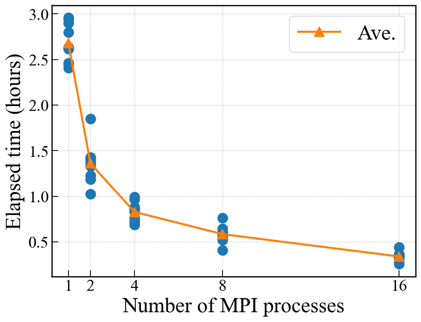
Random structure generation with MPI
Oct. 21 2023, update
Info
Requirements:
- CrySPY
1.1.0 1.2.3 or later - mpi4py
- MPI library (Open MPI, Intel MPI, MPICH, etc.)
Warning
1.1.0 <= CrySPY <=1.2.2 has a bug.
When you use bash (zsh) to run a job with MPI (e.g., jobcmd = zsh, jobfile = job_cryspy),
the MPI job does not run. There is no problem when you use a job scheduler (qsub, sbatch).
It has already fixed in version 1.2.3.
mpi4py
Install mpi4py if it is not already installed.
cryspy.in is the same as normal usage and does not need to be changed.
Here we try structure generation with MPI using the following settings:
[basic]
algo = RS
calc_code = soiap
tot_struc = 100
nstage = 1
njob = 2
jobcmd = zsh
jobfile = job_cryspy

[structure]
atype = Si
nat = 8

[soiap]
soiap_infile = soiap.in
soiap_outfile = soiap.out
soiap_cif = initial.cif

[option]
All except tot_struc, atype, and nat are irrelevant for structure generation and can be ignored here.
Run
If you want to generate structures with 4 MPI processes, just use mpiexec -n (with `-p`` option):
In 1.1.0 <= CrySPY <= 1.2.2, use (without `-p`` option)
If you submit the job with a job scheduler system, make the job file. Here is an example:
#!/bin/sh
#$ -cwd
#$ -V -S /bin/bash
#$ -N n_nproc
#$ -pe smp 4


mpirun -np $NSLOTS ~/.local/bin/cryspy
Please edit the location of the executable script cryspy.
Result
CrySPY simply divides the task (number of structures) by the number of processes:
- Rank 0: IDs 0 – 24
- Rank 1: IDs 25 – 49
- Rank 2: IDs 50 – 74
- Rank 3: IDs 75 – 99
CrySPY outputs the log in the order they are generated as follows:
2023/04/24 22:47:51
CrySPY 1.1.0
Start cryspy.py
Number of MPI processes: 4

Read input file, cryspy.in
Save input data in cryspy.stat

# --------- Generate initial structures
# ------ mindist
Si - Si 1.11
Structure ID     25 was generated. Space group: 138 --> 123 P4/mmm
Structure ID     75 was generated. Space group:  99 -->  99 P4mm
Structure ID      0 was generated. Space group: 127 --> 123 P4/mmm
Structure ID      1 was generated. Space group:  61 -->  61 Pbca
Structure ID     50 was generated. Space group:  38 -->  38 Amm2
Structure ID     51 was generated. Space group: 134 --> 123 P4/mmm
Structure ID     26 was generated. Space group: 111 --> 123 P4/mmm
Structure ID      2 was generated. Space group:   9 -->   9 Cc
Structure ID      3 was generated. Space group:  80 -->  80 I4_1
Structure ID      4 was generated. Space group: 107 --> 107 I4mm
Structure ID      5 was generated. Space group:  75 -->  75 P4
Structure ID     76 was generated. Space group: 108 --> 108 I4cm
Structure ID     77 was generated. Space group: 100 --> 100 P4bm
Structure ID     27 was generated. Space group: 207 --> 221 Pm-3m
However, the order in init_POSCARS is by structure ID since CrySPY outputs after all structures have been generated.
ID_0
1.0
   2.9636956737951818    0.0000000000000002    0.0000000000000002
   0.0000000000000000    2.9636956737951818    0.0000000000000002
   0.0000000000000000    0.0000000000000000    6.2634106638053080
Si
8
direct
  -0.1602734164607877   -0.1602734164607877   -0.0000000000000000 Si
   0.1602734164607877    0.1602734164607877    0.5000000000000000 Si
   0.6602734164607877    0.3397265835392123    0.7500000000000000 Si
   0.3397265835392122    0.6602734164607877    0.2500000000000000 Si
   0.4469739273741755    0.4469739273741755   -0.0000000000000000 Si
   0.5530260726258245    0.5530260726258244    0.5000000000000000 Si
   0.0530260726258245    0.9469739273741754    0.7500000000000000 Si
   0.9469739273741754    0.0530260726258245    0.2500000000000000 Si
ID_1
1.0
   7.2751506682509657    0.0000000000000004    0.0000000000000004
   0.0000000000000000    7.2751506682509657    0.0000000000000004
   0.0000000000000000    0.0000000000000000    5.1777634169924873
Si
8
direct
  -0.3845341807505553   -0.3845341807505553    0.4999999999999999 Si
   0.3845341807505553    0.3845341807505553    0.5000000000000000 Si
   0.3845341807505553   -0.3845341807505553    0.0000000000000000 Si
  -0.3845341807505553    0.3845341807505553   -0.0000000000000000 Si
   0.0000000000000000    0.5000000000000000    0.2500000000000000 Si
   0.5000000000000000    0.0000000000000000    0.7500000000000000 Si
   0.0000000000000000    0.5000000000000000    0.7500000000000000 Si
   0.5000000000000000    0.0000000000000000    0.2500000000000000 Si
ID_2
1.0
  -4.3660398676292269   -4.3660398676292269    0.0000000000000000
  -4.3660398676292269   -0.0000000000000003   -4.3660398676292269
   0.0000000000000000   -4.3660398676292269   -4.3660398676292269
Si
8
direct
   0.8700001548800920    0.8700001548800920    0.1299998451199080 Si
   0.1299998451199080    0.1299998451199080    0.8700001548800920 Si
   0.8700001548800920    0.1299998451199080    0.8700001548800920 Si
   0.1299998451199080    0.8700001548800920    0.1299998451199080 Si
   0.1299998451199080    0.8700001548800920    0.8700001548800920 Si
   0.8700001548800920    0.1299998451199080    0.1299998451199080 Si
   0.7500000000000000    0.7500000000000000    0.7500000000000000 Si
   0.2500000000000000    0.2500000000000000    0.2500000000000000 Si
Note
Except for the random structure generation part, there is no point in using MPI because it is not parallelized.
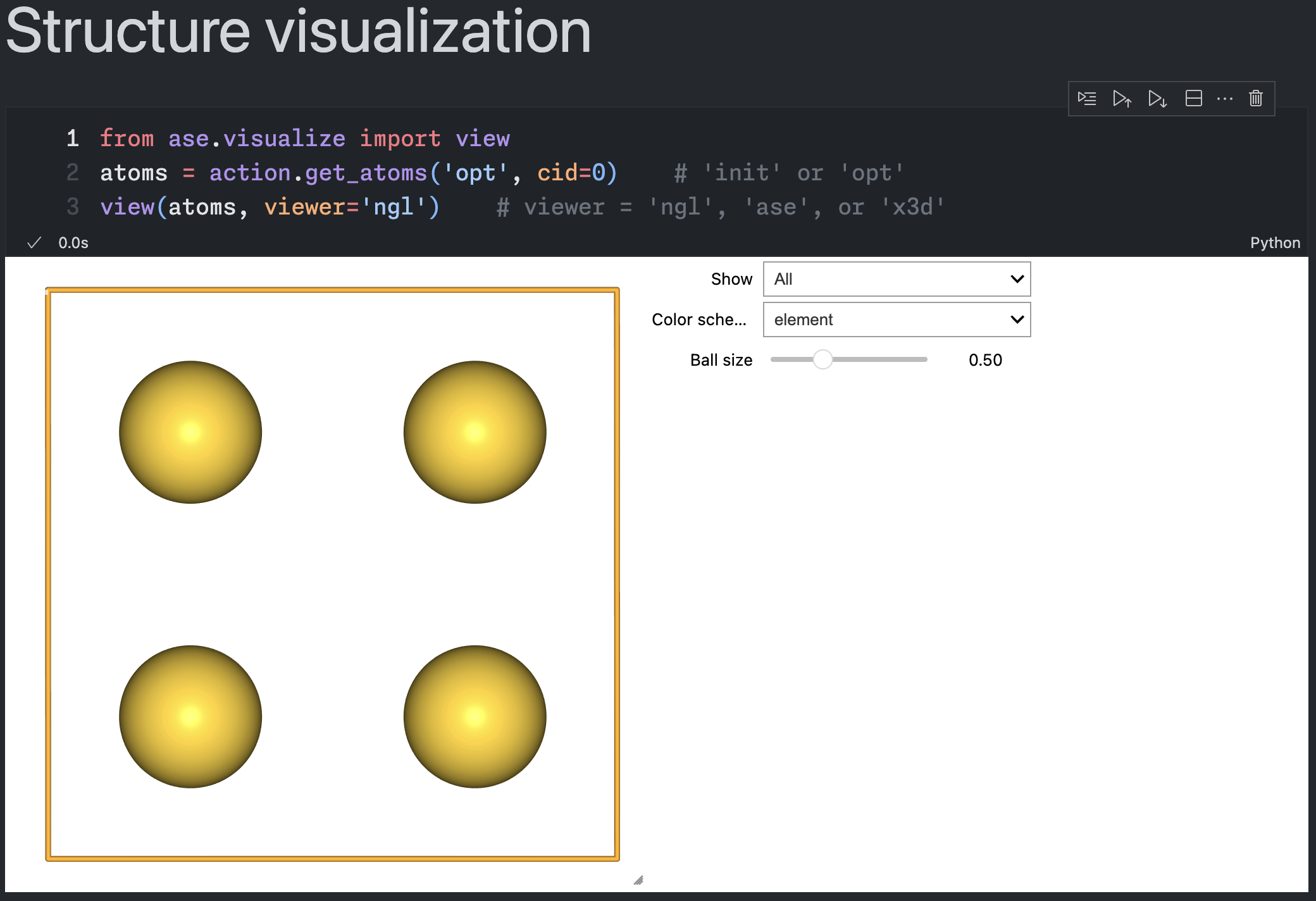
Interactive mode (Jupyter Notebook)
2025 March 6
Info
Requirements:
- CrySPY 1.4.0 or later
- Jupyter
- Structure optimization software compatible with ASE (e.g., machine learning potentials).
- nglview (optional)
Preparation
When CrySPY is installed, ASE is automatically installed as well.
Set up Jupyter to be usable on a workstation or local PC.
In this tutorial, Pure Python EMT calculator is used for structure optimization. Note that the accuracy of the EMT potential is poor, as it is intended for demonstration purposes only.
The example notebook also includes code for using the machine learning potential CHGNet.
If you want to try CHGNet, make sure to install it in advance using pip.
Move to your working directory, and copy the example files by one of the following methods.
Even in interactive mode, cryspy.in is used as the input file.
The calc_in directory is not used in interactive mode.
You can refer to the examples of cryspy.in in the input_examples directory.
Here, the following cryspy.in using EA-vc will be used.
For more details on EA-vc, refer to the EA-vc tutorial.
[basic]
algo = EA-vc
calc_code = ASE
nstage = 1
njob = 10
jobcmd = zsh
jobfile = job_cryspy

[structure]
atype = Cu Au
ll_nat = 0 0
ul_nat = 8 8

[ASE]
ase_python = ase_in.py

[EA]
n_pop = 20
n_crsov = 5
n_perm = 2
n_strain = 2
n_rand = 2
n_add = 3
n_elim = 3
n_subs = 3
target = random
n_elite = 2
n_fittest = 10
slct_func = TNM
t_size = 2
maxgen_ea = 5
end_point = 0.0 0.0

[option]
Notebook
Open cryspy_interactive.ipynb and execute the cells from the top.
Check current working directory
The first cell only checks the files and the contents of cryspy.in.
!pwd
print()
!ls
print()
!cat cryspy.in
Import
Ignore the commented-out sections this time and execute the cell that imports the core libraries for CrySPY’s interactive mode.
# ---------- import
from cryspy.interactive import action
Initialize CrySPY
This cell corresponds to a standard initial run. It reads cryspy.in and generates the initial structures.
# ---------- initial structure generation
action.initialize()
Set calculator
This cell sets the ASE calculator. Here, ASE’s EMT is used.
# ---------- EMT in ASE
from ase.calculators.emt import EMT
calculator = EMT()

# ---------- CHGNet
#from chgnet.model import CHGNetCalculator
#calculator = CHGNetCalculator()
Restart CrySPY
Executing this cell starts the optimization of the previously generated initial structures.
In interactive mode, structure optimization calculations are performed sequentially, one by one. A progress bar is also displayed during the process.
# ---------- structure optimization
action.restart(
    njob=20,    # njob=0: njob in cryspy.in will be used
    calculator=calculator,
    optimizer='BFGS',    # 'FIRE', 'BFGS' or 'LBFGS'
    symmetry=True,       # default: True
    fmax=0.01,           # default: 0.01 eV/Å
    steps=2000,          # default: 2000
)
- njob: The number of structures to be optimized in a single execution. If set to 0, the value specified in
cryspy.in is used. - calculator: Assign the previously set calculator.
- optimizer: Select from
FIRE, BFGS, or LBFGS. Specify as a string. - symmetry: If True, structure optimization is performed while preserving symmetry.
- fmax: The maximum atomic force (eV/Å) used for convergence criteria.
- steps: Maximum optimization steps.
If the njob value is set to a small number, execute this cell multiple times to complete the optimization of all initial structures.
When using EA-vc, the following message will be displayed upon completion.
Executing this cell again will trigger generational turnover.
Once the next-generation structures are generated, continue executing this cell repeatedly in the same manner.
Show results
Running this cell allows you to display files such as cryspy_rslt_energy_asc.
# ---------- show results
#!cat ./data/cryspy_rslt    # Order of structure optimization completion
!cat ./data/cryspy_rslt_energy_asc    # show energy ascending order
#!sed -n 2,4p ./data/cryspy_rslt    # show i--jth lines
#!tail -n 5 ./data/cryspy_rslt    # show last 5 lines
Structure visualization
You can interactively visualize both the initial and optimized structures.
from ase.visualize import view
atoms = action.get_atoms('opt', cid=0)    # 'init' or 'opt'
view(atoms, viewer='ngl')    # viewer = 'ngl', 'ase', or 'x3d'
Changing opt to init in action.get_atoms('opt', cid=0) allows you to check the initial structure.
The cid parameter specifies the structure ID.
Since this utilizes ASE’s functionality, the viewer option supports ngl, ase, and x3d.
To use ngl, you need to install nglview, so make sure to install it via pip in advance.

Energy plot for RS, EA
For random search (RS) and evolutionary algorithm (EA), an energy graph shown below can be displayed.
In the case of EA-vc, direct energy comparison is not possible due to differences in the number of atoms, so the convex hull plot, discussed later, is used instead.
fig, ax = action.plot_E(
              title=None,
              ymax=2.0,
              ymin=-0.5,
              markersize=12,
              marker_edge_width=1.0,
              marker_edge_color='black',
              alpha=1.0,
          )
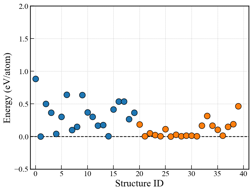
Convex hull plot for EA-vc
Interactive plot using Plotly
For EA-vc, an interactive convex hull plot using Plotly is available.
When CrySPY is installed, Plotly is automatically installed as well.
This convex hull plot utilizes pymatgen’s functionality.
action.interactive_plot_convex_hull(cgen=None, show_unstable=0.2, ternary_style='2d')
- cgen: Which generation’s data to plot up to. If None, data will be plotted up to the latest generation.
- show_unstable: The maximum hull distance value to display on the plot
- ternary_style
- Binary system: ternary_style = ‘2d’
- Ternary system: ternary_style = ‘2d’, ‘3d’
- Quaternary system: ternary_style = ‘3d’
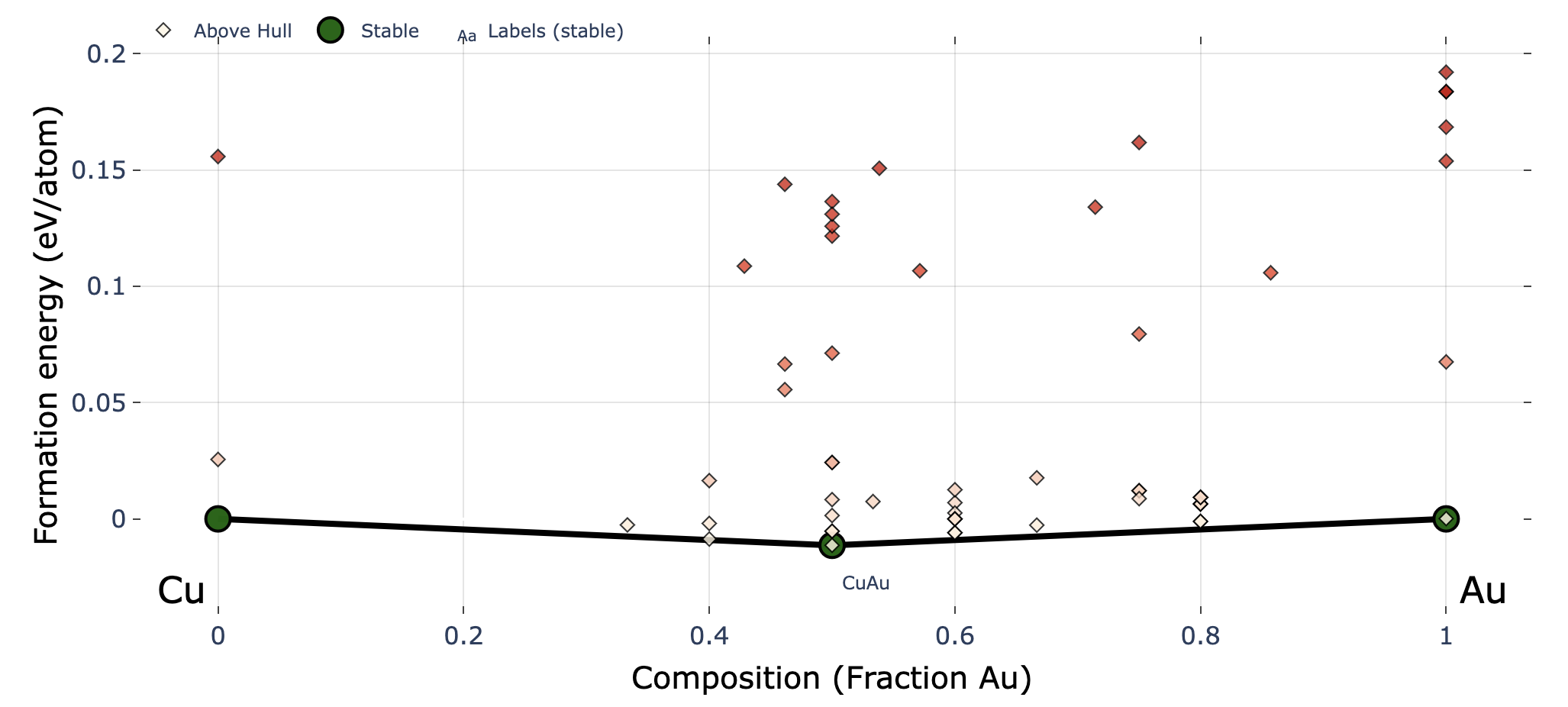
When performing calculations with ternary or quaternary systems instead of binary systems, you can obtain the following interactive plots.
From left to right:
- Ternary system (ternary_style = ‘2d’)
- Ternary system (ternary_style = ‘3d’)
- Quaternary system (ternary_style = ‘3d’)
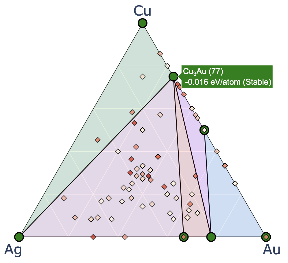
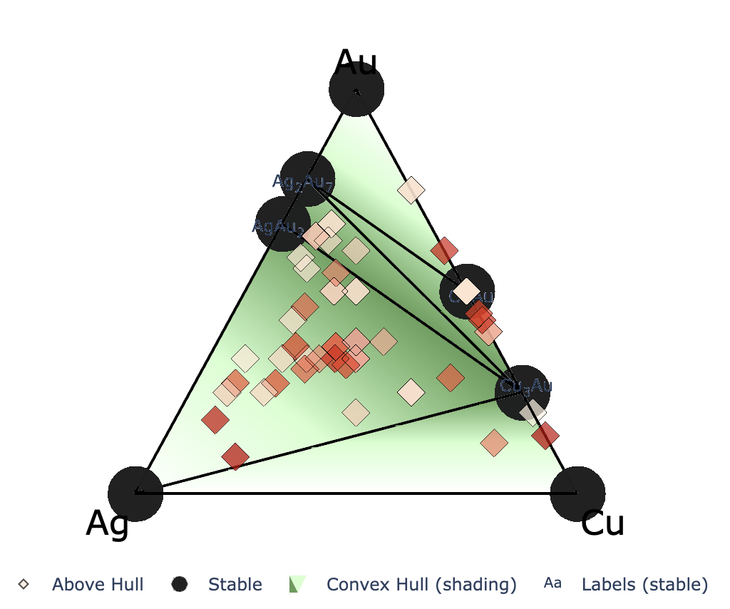
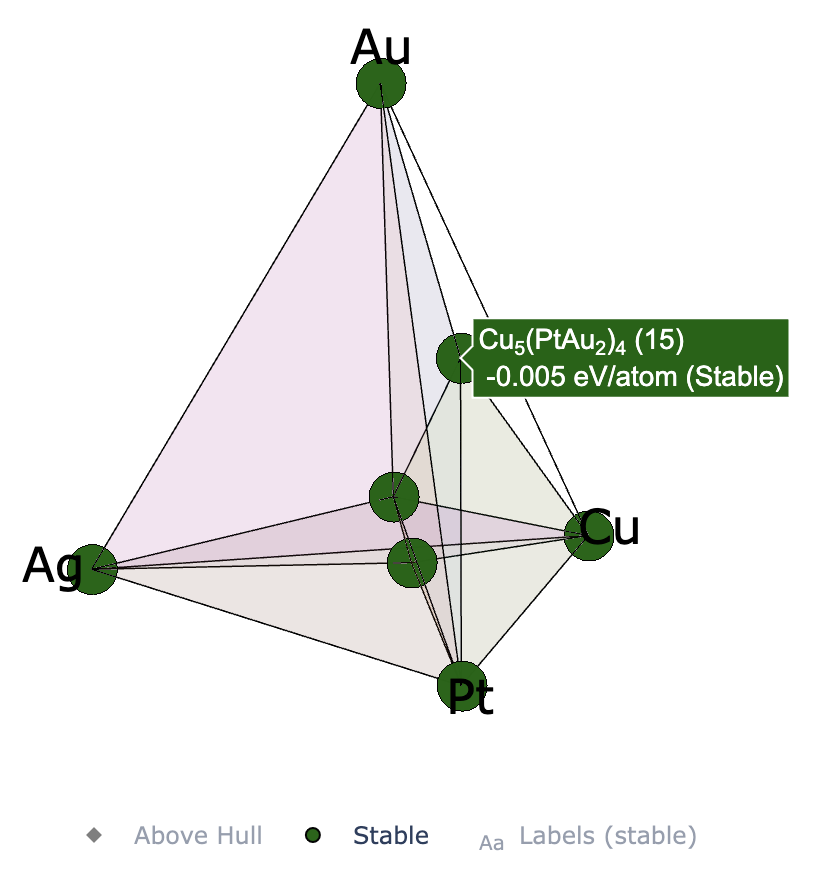
Binary system using matplotlib
Running this cell plots the binary convex hull using matplotlib.
fig, ax = action.plot_convex_hull_binary(
              cgen=None,
              show_max=0.2,
              label_stable=True,
              vmax=0.2,
              bottom_margin=0.02,
          )
fig    # to show plot in jupyter
- cgen: Which generation’s data to plot up to. If None, data will be plotted up to the latest generation.
- show_max: The maximum formation energy to display on the plot
- label_stable: Whether to display the labels (compositions) of stable structures
- vmax: The maximum hull distance in the color bar
- bottom_margin: Bottom margin of y-axis
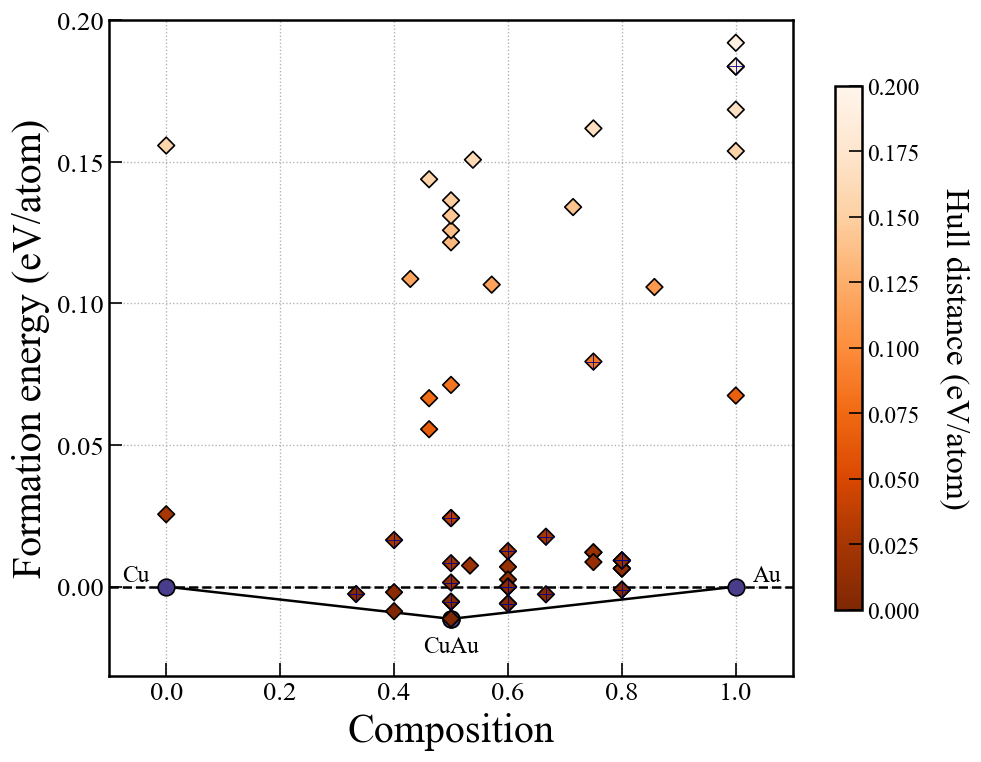
Ternary system using matplotlib
If exploring a ternary system, running this cell will generate a convex hull plot using matplotlib.
fig, ax = action.plot_convex_hull_ternary(
              cgen=None,
              show_max=0.2,
              label_stable=True,
              vmax=0.2,
          )
fig    # to show plot in jupyter
- cgen: Which generation’s data to plot up to. If None, data will be plotted up to the latest generation.
- show_max: The maximum formation energy to display on the plot
- label_stable: Whether to display the labels (compositions) of stable structures
- vmax: The maximum hull distance in the color bar
For example, the following plot can be obtained.