チュートリアル

情報

初心者の方はランダムサーチから始めると良い．Exampleファイルはこちら –> cryspy_utility.

ランダムサーチ (RS)

情報

ASE は初心者にとって始めやすいツールである． CrySPYのインストール時に，ASEも自動的にインストールされるためである．高い精度はないが，非常に軽量で高速な原子間ポテンシャルを備えており，ノートPCなどの低スペックな環境でも動作確認に適している．

入力ファイルの準備

下記のどれか一つに従い，その後CrySPY実行のセクションに移ること．

CrySPY実行

ASE on your local PC

2025年7月11日更新 v1.4.2

ASEは様々なコードのインターフェースを提供しているPythonライブラリであり， Pure Python EMT calculatorというシンプルなEMTの計算も実行できる．CrySPYさえインストールしてあれば，精度はともかく簡単に計算できるので，CrySPYのテストにちょうど良い．

このチュートリアルでは，MacやLinuxなどのOSのローカルPCを用いてCu 8原子の構造探索を試す．

Assumption

ここでは次のような条件を想定している：

CrySPY 1.2.0 or later in your local PC
CrySPY job filename: job_cryspy
ase input filename: ase_in.py

Input files

どこか適当なワーキングディレクトリに移動して，まずはexampleをコピーしてくる．下記のどちらからコピーしてきても良い．

Download from CrySPY_utility/examples/ase_Cu8_RS
Copy from CrySPY utility that you installed

cd ase_Cu8_RS
tree

.
├── calc_in
│   ├── ase_in.py
│   └── job_cryspy
└── cryspy.in

cryspy.in

cryspy.inはCrySPYの入力ファイル．

[basic]
algo = RS
calc_code = ASE
tot_struc = 5
nstage = 1
njob = 5
jobcmd = zsh
jobfile = job_cryspy

[structure]
atype = Cu
nat = 8

[ASE]
ase_python = ase_in.py

[option]

[basic] セクションのjobcmd = zshは環境に合わせてjobcmd = shやjobcmd = bash等に変更する． CrySPYは内部でバックグラウンドジョブとしてzsh job_cryspyを実行する．

ASEを使う場合は，[ASE]セクションが必要．下記の二つのファイル名は好きなように変えても良い．

jobfile: job_cryspy
ase_python: ase_in.py

他の入力変数については後で説明を行う．

calc_in directory

ASEのジョブファイルや入力ファイルはこのディレクトリに準備する．

Job file

ジョブファイルの名前はcryspy.inのjobfileに一致させる必要がある．ジョブファイルの例は下記の通り．

#!/bin/sh

# ---------- ASE
python3 ase_in.py

ase_in.pyというファイル名も自由に変えられるが， cryspy.inのase_pythonの値と一致させておく必要がある． ~~CrySPYではジョブファイルの最後の行はsed -i -e ‘3 s/^.*$/done/’ stat_jobとしておくルールになっている．~~ バージョン1.4.2からCrySPYがジョブファイルの末尾に自動的に下記を追記するようになった．（参考：機能 > ジョブファイルの自動書き換え）

# ---------- CrySPY
sed -i -e '3s/^sub.*/done/' stat_job

メモ

1.4.2より古いバージョンでは，ジョブファイルの最後の行はsed -i -e '3s/^sub.*/done/' stat_jobと書いておくルールになっている．自分でsedコマンド文を書いたジョブファイルを1.4.2以上のバージョンで使用しても2回実行されるだけなので問題はない．
上記sedコマンドの意味は，stat_jobというファイルの3行目のsubから始まる部分をdoneに変える処理．

ヒント

（詳細：機能 > ジョブファイルの自動書き換え）
CrySPYのジョブファイルのCrySPY_IDという文字列は自動的に構造IDに置き換わるようになっている． PBSやSLURMといったジョブスケジューラーを使う場合，ジョブ名にCrySPY_IDと書いておくとどの構造のジョブなのかが分かり便利である．例えば，PBSでは#PBS -N Si_CrySPY_IDのように書いておくと，ジョブをサブミットする際，#PBS -N Si_10のように置き換わる．注意点として，ジョブ名を数字から始めるとエラーとなることが多いので，Si_のように何か文字列を頭につけておくこと．

Input for ASE

ステージ数(nstage in cryspy.in)に応じた数のインプットファイルが必要となる．インプットファイル名の先頭にx_，または語尾に_xをつけて準備する．ここでxはステージ数．

CrySPYが探すインプットファイル名の優先順位は以下の通り．

x_ase_in.py
ase_in.py_x
ase_in.py

各ステージで共通のインプットを使用するのであればx_や_xを省略できる．

このASEのチュートリアルではnstage = 1を用いるので，ASEのインプットファイルはase_in.pyの一つだけでよい．x_や_xを省略したファイルを準備している． ase_in.pyは例えば下記の通り（ASEの使い方の詳細は公式のドキュメントを見ること）．

from ase.constraints import FixSymmetry
from ase.filters import FrechetCellFilter
from ase.calculators.emt import EMT
from ase.optimize import BFGS
from ase.io import read, write

# ---------- input structure
# CrySPY outputs 'POSCAR' as an input file in work/xxxxxx directory
atoms = read('POSCAR', format='vasp')

# ---------- setting and run
atoms.calc = EMT()
atoms.set_constraint([FixSymmetry(atoms)])
cell_filter = FrechetCellFilter(atoms, hydrostatic_strain=False)
opt = BFGS(cell_filter)

# ---------- run
converged = opt.run(fmax=0.01, steps=2000)

# ---------- rule in ASE interface
# output file for energy: 'log.tote' in eV/cell
#                         CrySPY reads the last line of 'log.tote' file
# outimized structure: 'CONTCAR' file in vasp format
# check_opt: 'out_check_opt' file ('done' or 'not yet')
#                         CrySPY reads the last line of 'out_check_opt' file

# ------ energy
e = cell_filter.atoms.get_total_energy()    # eV/cell
with open('log.tote', mode='w') as f:
    f.write(str(e))

# ------ struc
opt_atoms = cell_filter.atoms.copy()
opt_atoms.set_constraint(None)    # remove constraint for pymatgen
write('CONTCAR', opt_atoms, format='vasp', direct=True)

# ------ check_opt
with open('out_check_opt', mode='w') as f:
    if converged:
        f.write('done\n')
    else:
        f.write('not yet\n')

ASEはVASPやQEなどと違って，入力ファイル（python script）は自分で書くことになるので自由度がある． CrySPYでは3つのルールを設けている．

エネルギーはeV/cellの単位でlog.toteというファイルに出力する．CrySPYはこのファイルの最後の行を読む．
最適化後の構造データはCONTCARというファイルにVASPフォーマットで出力する．
最適化の収束判定結果をout_check_optというファイルにdoneかnot_yetで書き込む．CrySPYはこのファイルの最後の行を読む．

CrySPY実行

ここまで準備ができたらCrySPY実行へ進む．

soiap on your local PC

情報

ここに書いてある内容は少し古いので，最近のチュートリアルはチュートリアル > ランダムサーチ（RS） > ASE on your local PCを見ること．このページの内容も動作には問題ないはず．

2025年3月6日更新

soiapは原子間ポテンシャルを使用した計算ができるソフトウェアであり，計算が軽いのでCrySPYのテストにちょうど良い． soiapのインストールや詳細はinstructionsを参照．

このチュートリアルでは，MacやLinuxのローカルPC上でCrySPYを試す．テストシステムはSi 8原子．

Assumption

ここでは次のような条件を想定している：

(only version 0.10.3 or earlier) CrySPY main script: ~/CrySPY_root/CrySPY-0.9.0/cryspy.py
CrySPY job filename: job_cryspy
soiap executable file: ~/local/soiap-0.3.0/src/soiap
soiap input filename: soiap.in
soiap output filename: soiap.out
soiap input structure filename: initial.cif

Input files

どこか適当なワーキングディレクトリに移動して，まずはexampleをコピーしてくる．下記のどちらからコピーしてきても良い．

Download from Cryspy_utility/examples/soiap_Si8_RS
Copy from CrySPY utility that you installed
(only version 0.10.3 or earlier) cp -r ~/CrySPY_root/CrySPY-0.9.0/example/v0.9.0/soiap_RS_Si8 .

cd soiap_RS_Si8
tree

.
├── calc_in
│   ├── job_cryspy
│   └── soiap.in_1
└── cryspy.in

cryspy.in

cryspy.inがCrySPYの入力ファイル．

[basic]
algo = RS
calc_code = soiap
tot_struc = 5
nstage = 1
njob = 2
jobcmd = zsh
jobfile = job_cryspy

[structure]
atype = Si
nat = 8

[soiap]
soiap_infile = soiap.in
soiap_outfile = soiap.out
soiap_cif = initial.cif

[option]

soiapを使う場合は[soiap]セクションが必要となる．下記のファイル名は好きなように変えても良い．

jobfile
soiap_infile
soiap_outfile
soiap_cif

他の入力変数については後で説明を行う．

calc_in directory

soiapのジョブファイルや入力ファイルはこのディレクトリに準備する．

Job file

ジョブファイルの名前はcryspy.inのjobfileに一致させる必要がある．ジョブファイルの例は下記の通り．

#!/bin/sh

# ---------- soiap
EXEPATH=/path/to/soiap
$EXEPATH/soiap soiap.in 2>&1 > soiap.out

# ---------- CrySPY
sed -i -e '3 s/^.*$/done/' stat_job

/path/to/soiapはsoiapの実行ファイルのpathに変えること．入力ファイル（soiap.in）と出力ファイル（soiap.out）はcryspy.inで指定したsoiap_infileとsoiap_outfileに合わせること．最後の行以外は普段使っているようなジョブスクリプトで良いが， CrySPYではジョブファイルの最後の行はsed -i -e '3 s/^.*$/done/' stat_jobとしておくルールになっている．

メモ

ジョブファイルの最後の行はsed -i -e '3 s/^.*$/done/' stat_jobと書いておく．

ヒント

CrySPYのジョブファイルのCrySPY_IDという文字列は自動的に構造IDに置き換わるようになっている． PBSやSLURMといったジョブスケジューラーを使う場合，ジョブ名にCrySPY_IDと書いておくとどの構造のジョブなのかが分かり便利である．例えば，PBSでは#PBS -N Si_CrySPY_IDのように書いておくと，ジョブをサブミットする際，#PBS -N Si_10のように置き換わる．注意点として，ジョブ名を数字から始めるとエラーとなることが多いので，Si_のように何か文字列を頭につけておくこと．

Input for soiap

ステージ数(nstage in cryspy.in)に応じた数のインプットファイルが必要となる．インプットファイル名の語尾に_xをつけて準備する．ここでxはステージ数．

soiapのチュートリアルではnstage = 1を用いるので，インプットファイルはsoiap.in_1の一つだけが必要． soiap.in_1は例えば下記の通り．

crystal initial.cif ! CIF file for the initial structure
symmetry 1 ! 0: not symmetrize displacements of the atoms or 1: symmetrize

md_mode_cell 3 ! cell-relaxation method
               ! 0: FIRE, 2: quenched MD, or 3: RFC5
number_max_relax_cell 100 ! max. number of the cell relaxation
number_max_relax 1 ! max. number of the atom relaxation
max_displacement 0.1 ! max. displacement of atoms in Bohr

external_stress_v 0.0 0.0 0.0 ! external pressure in GPa

th_force 5d-5 ! convergence threshold for the force in Hartree a.u.
th_stress 5d-7 ! convergence threshold for the stress in Hartree a.u.

force_field 1 ! force field
              ! 1: Stillinger-Weber for Si, 2: Tsuneyuki potential for SiO2,
              ! 3: ZRL for Si-O-N-H, 4: ADP for Nd-Fe-B, 5: Jmatgen, or
              ! 6: Lennard-Jones

1行目に書く初期構造ファイル（initial.cif）はcryspy.inのsoiap_cifの値と揃える．

CrySPY実行

ここまで準備ができたらCrySPY実行へ進む．

VASP

2025年7月12日　更新

このチュートリアルでは，PBSなどのジョブスケジューラーを備えたPCクラスターを想定してCrySPYを試す．第一原理計算のVASPを用いて，Na8Cl8（16原子）の構造探索を行う．

Assumption

ここでは次のような条件を想定している：

CrySPY 1.2.0 or later in your PC cluster
CrySPY job command: qsub
CrySPY job filename: job_cryspy
executable file, vasp_std in your PC cluster

Input files

どこか適当なワーキングディレクトリに移動して，まずはexampleをコピーしてくる．下記のどちらからコピーしてきても良い．

Download from Cryspy_utility/examples/vasp_Na8Cl8_RS
Copy from CrySPY utility that you installed

cd vasp_Na8Cl8_RS
tree

.
├── calc_in
│   ├── 1_INCAR
│   ├── 2_INCAR
│   ├── POTCAR_dummy
│   └── job_cryspy
└── cryspy.in

cryspy.in

cryspy.inはCrySPYの入力ファイル．

[basic]
algo = RS
calc_code = VASP
tot_struc = 5
nstage = 2
njob = 2
jobcmd = qsub
jobfile = job_cryspy

[structure]
atype = Na Cl
nat = 8 8
mindist_1 = 2.5 1.5
mindist_2 = 1.5 2.5

[VASP]
kppvol = 40 80

[option]

[basic] セクションのjobcmd = qsubは環境に合わせて変更する． CrySPYは内部でバックグラウンドジョブとしてqsub job_cryspyを実行する．下記のファイル名は好きなように変えても良い．

jobfile

構造最適化計算はステージ制を採用しており，ここではnstage = 2を用いている．例えば，最初のステージでは，セルを固定し内部座標だけ緩和する設定で，k点も少ない計算を実行し，2ステージ目でセルも含めてフルに構造緩和して，精度も高めるようなことが可能となっている．

VASPを使う場合は，[VASP]セクションが必要．ここでは各ステージにおけるk点のグリッド密度（Å^-3）をkppvolに指定する必要がある．

情報

kppvolの詳細はこちら –> Input file > Kpoint

他のインプット変数に関しては後ほど説明する．

calc_in directory

ジョブファイルやVASPのインプットをこのディレクトリに置く．

Job file

ジョブファイルの名前はcryspy.inのjobfileに一致させる必要がある．ジョブファイルの例は下記の通り．

#!/bin/sh
#$ -cwd
#$ -V -S /bin/bash
####$ -V -S /bin/zsh
#$ -N Na8Cl8_CrySPY_ID
#$ -pe smp 20
####$ -q ibis1.q
####$ -q ibis2.q
####$ -q ibis3.q
####$ -q ibis4.q

# ---------- vasp
VASPROOT=/usr/local/vasp/vasp.6.4.2/bin
mpirun -np $NSLOTS $VASPROOT/vasp_std

VASPROOTは環境に合わせて変更する．普段VASPのジョブを流しているジョブファイルを使えば良い． ~~CrySPYではジョブファイルの最後の行はsed -i -e ‘3 s/^.*$/done/’ stat_jobとしておくルールになっている．~~ バージョン1.4.2からCrySPYがジョブファイルの末尾に自動的に下記を追記するようになった．（参考：機能 > ジョブファイルの自動書き換え）

# ---------- CrySPY
sed -i -e '3s/^sub.*/done/' stat_job

メモ

ヒント

Input for VASP

CrySPYが探すインプットファイル名の優先順位は以下の通り．

x_INCAR
INCAR_x
INCAR

各ステージで共通のインプットを使用するのであればx_や_xを省略できる．

今はnstage = 2を用いているので，1_INCAR_1と2_INCARが必要となる．ここでは，1_INCARはセルを固定して内部座標だけ緩和する設定，2_INCARはセルも含めてフルに緩和する設定になっている．

1_INCAR

SYSTEM = NaCl
!!!LREAL = Auto
Algo = Fast
NSW = 40

LWAVE = .FALSE.
!LCHARG = .FALSE.

ISPIN =  1

ISMEAR = 0
SIGMA = 0.1

IBRION = 2
ISIF = 2

EDIFF = 1e-5
EDIFFG = -0.01

2_INCAR

SYSTEM = NaCl
!!LREAL = Auto
Algo = Fast
NSW = 200

ENCUT = 341

!!LWAVE = .FALSE.
!!LCHARG = .FALSE.


ISPIN =  1

ISMEAR = 0
SIGMA = 0.1

IBRION = 2
ISIF = 3

EDIFF = 1e-5
EDIFFG = -0.01

CrySPYはPOSCARとKPOINTSファイルを自動生成する． POTCARファイルはユーザーが準備する必要がある．このexampleに含まれているPOTCARは空のファイルなので，各自で準備すること．

警告

exampleに含まれているPOTCARは空のファイル．配布できない．

CrySPY実行

ここまで準備ができたらCrySPY実行に進む．

QE

2025年7月18日　更新

このチュートリアルでは，PBSなどのジョブスケジューラーを備えたPCクラスターを想定してCrySPYを試す．第一原理計算のQUANTUM ESPRESSOを用いて，Si 8原子の構造探索を行う．

Assumption

ここでは次のような条件を想定している：

CrySPY job command: qsub
CrySPY job filename: job_cryspy
QE executable file: /usr/local/qe-6.5/bin/pw.x
QE input filename: pwscf.in
QE output filename: pwscf.out

Input files

どこか適当なワーキングディレクトリに移動して，まずはexampleをコピーしてくる．下記のどちらからコピーしてきても良い．

Download from CrySPY_utility/examples/qe_Si8_RS
Copy from CrySPY utility that you installed

cd QE_RS_Si8
tree

.
├── calc_in
│   ├── job_cryspy
│   ├── 1_pwscf.in
│   └── 2_pwscf.in
└── cryspy.in

cryspy.in

cryspy.inはCrySPYの入力ファイル．

[basic]
algo = RS
calc_code = QE
tot_struc = 5
nstage = 2
njob = 2
jobcmd = qsub
jobfile = job_cryspy

[structure]
atype = Si
nat = 8

[QE]
qe_infile = pwscf.in
qe_outfile = pwscf.out
kppvol =  40  80

[option]

[basic] セクションのjobcmd = qsubは環境に合わせて変更する． CrySPYは内部でバックグラウンドジョブとしてqsub job_cryspyを実行する．

QEを使う場合は，[QE]セクションが必要．ここでは各ステージにおけるk点のグリッド密度（Å^-3）をkppvolに指定する必要がある．

情報

kppvolの詳細はこちら –> Input file > Kpoint

下記のファイル名は好きなように変えても良い．

jobfile
qe_infile
qe_outfile

他のインプット変数に関しては後ほど説明する．

calc_in directory

ジョブファイルやQEのインプットをこのディレクトリに置く．

Job file

ジョブファイルの名前はcryspy.inのjobfileに一致させる必要がある．ジョブファイルの例は下記の通り．

#!/bin/sh
#$ -cwd
#$ -V -S /bin/bash
####$ -V -S /bin/zsh
#$ -N Si8_CrySPY_ID
#$ -pe smp 20
####$ -q ibis1.q
####$ -q ibis2.q

mpirun -np $NSLOTS /path/to/pw.x < pwscf.in > pwscf.out


if [ -e "CRASH" ]; then
    sed -i -e '3 s/^.*$/skip/' stat_job
    exit 1
fi

/path/to/pw.xは環境に合わせて変更する．入力（pwscf.in）出力（pwscf.out）ファイルの名前は好きに変えて良いが，cryspy.inのqe_infileとqe_outfileに合わせる必要がある．普段QEのジョブを流しているジョブファイルを使えば良い． ~~CrySPYではジョブファイルの最後の行はsed -i -e ‘3 s/^.*$/done/’ stat_jobとしておくルールになっている．~~ バージョン1.4.2からCrySPYがジョブファイルの末尾に自動的に下記を追記するようになった．（参考：機能 > ジョブファイルの自動書き換え）

# ---------- CrySPY
sed -i -e '3s/^sub.*/done/' stat_job

メモ

ヒント

Input for QE

CrySPYが探すインプットファイル名の優先順位は以下の通り．

x_pwscf.in
pwscf.in_x
pwscf.in

各ステージで共通のインプットを使用するのであればx_や_xを省略できる．

今はnstage = 2を用いているので，1_pwscf.inと2_pwscf.inが必要となる．ここでは，1_pwscf.inはセルを固定して内部座標だけ緩和する設定，2_pwscf.inはセルも含めてフルに緩和する設定になっている．

1_pwscf.in

 &control
    title = 'Si8'
    calculation = 'relax'
    nstep = 100
    restart_mode = 'from_scratch',
    pseudo_dir = '/usr/local/pslibrary.1.0.0/pbe/PSEUDOPOTENTIALS/'
    outdir='./out.d/'
 /

 &system
    ibrav = 0
    nat = 8
    ntyp = 1
    ecutwfc = 44.0
    occupations = 'smearing'
    degauss = 0.01
 /

 &electrons
 /

 &ions
 /

 &cell
 /

ATOMIC_SPECIES
  Si  28.086  Si.pbe-n-kjpaw_psl.1.0.0.UPF

2_pwscf.in

 &control
    title = 'Si8'
    calculation = 'vc-relax'
    nstep = 200
    restart_mode = 'from_scratch',
    pseudo_dir = '/usr/local/pslibrary.1.0.0/pbe/PSEUDOPOTENTIALS/'
    outdir='./out.d/'
 /

 &system
    ibrav = 0
    nat = 8
    ntyp = 1
    ecutwfc = 44.0
    occupations = 'smearing'
    degauss = 0.01
 /

 &electrons
 /

 &ions
 /

 &cell
 /

ATOMIC_SPECIES
  Si  28.086  Si.pbe-n-kjpaw_psl.1.0.0.UPF

pseudo_dirは各自の環境に合わせて変更する． Inputs for structure data and k-point such as インプットファイルのATOMIC_POSITIONSとK_POINTSはCrySPYがpymatgenを用いて自動生成するのでユーザーが書く必要はない．

CrySPY実行

ここまで準備ができたらCrySPY実行に進む．

OpenMX

Coming soon.

LAMMPS

Coming soon.

Check cryspy.in

2025年6月16日更新

詳細は入力ファイルのページも見ること．

cryspy.inをもう一度チェックしてみよう．ここでの例は選んだcalc_codeに応じて，準備したものと少し異なるかもしれない．

[basic]
algo = RS
calc_code = ASE
tot_struc = 5
nstage = 1
njob = 5
jobcmd = zsh
jobfile = job_cryspy

[structure]
atype = Cu
nat = 8

[ASE]
ase_python = ase_in.py

[option]

[basic] section

algo: アルゴリズム．ランダムサーチの場合はRSを使う．
calc_code: 構造最適化のコード． VASP, QE, OMX, soiap, LAMMPS, ASEから選択．
tot_struc: 構造数．この場合初回実行で5構造ランダムに生成される．
nstage: ステージ数
njob: 同時にサブミットするジョブの数．この例では2つのスロットを設定，言い換えると，2構造ずつ最適化を行う．
jobcmd: ジョブを実行または投入するコマンド． bash, zsh, qsubなど
jobfile: ジョブファイルのファイル名

[structure] section

atype: Atom type. Na8Cl8の例： atype = Na Cl.
nat: atypeに応じた原子数． Na8Cl8の例： nat = 8 8

Script to run

メモ

For version 1.0.0 or later, skip this page. The executable script is automatically installed.

Assumption

Here, we assume the following condition:

CrySPY main script: ~/CrySPY_root/CrySPY-0.9.0/cryspy.py

Make script

Let’s make a convenient shell script to avoid typing long commands over and over again. Here, we create the script, cryspy (any file name will do).

$ emacs cryspy
$ chmod 744 cryspy
$ cat cryspy

#!/bin/sh

python3 -u ~/CrySPY_root/CrySPY-0.9.0/cryspy.py 1>> log 2>> err

-u option (unbuffered option) can be omitted.

You can put this script in your $PATH, or just use like bash ./cryspy.

Firsrt run

2025 March 6, updated

Make sure you have the following in your working directory.

calc_in/
(cryspy)
cryspy.in

$ ls
calc_in/  cryspy.in

Then, run CyrSPY!

cryspy

If you use old version (0.10.3 or earlier):

bash ./cryspy

At the first run, CrySPY goes into structure generation mode. CrySPY stops after 5 structure generation.

If it worked properly, the following output appears on the screen:

[2025-03-06 18:52:21,495][cryspy_init][INFO] 


Start CrySPY 1.4.0


[2025-03-06 18:52:21,495][cryspy_init][INFO] # ---------- Library version info
[2025-03-06 18:52:21,495][cryspy_init][INFO] pandas version: 2.2.2
[2025-03-06 18:52:21,495][cryspy_init][INFO] pymatgen version: 2025.1.24
[2025-03-06 18:52:21,495][cryspy_init][INFO] pyxtal version: 1.0.6
[2025-03-06 18:52:21,495][cryspy_init][INFO] # ---------- Read input file, cryspy.in
[2025-03-06 18:52:21,496][write_input][INFO] [basic]
[2025-03-06 18:52:21,496][write_input][INFO] algo = RS
[2025-03-06 18:52:21,496][write_input][INFO] calc_code = ASE
[2025-03-06 18:52:21,496][write_input][INFO] tot_struc = 5
[2025-03-06 18:52:21,496][write_input][INFO] nstage = 1
[2025-03-06 18:52:21,496][write_input][INFO] njob = 2
[2025-03-06 18:52:21,496][write_input][INFO] jobcmd = zsh
[2025-03-06 18:52:21,496][write_input][INFO] jobfile = job_cryspy
...
(omitted)
...
[2025-03-06 18:52:21,497][rs_gen][INFO] # ---------- Initial structure generation
[2025-03-06 18:52:21,497][rs_gen][INFO] # ------ mindist
[2025-03-06 18:52:21,498][struc_util][INFO] Cu - Cu: 1.32
[2025-03-06 18:52:21,498][rs_gen][INFO] # ------ generate structures
[2025-03-06 18:52:21,519][gen_pyxtal][INFO] Structure ID      0: (8,) Space group:  31 -->  31 Pmn2_1
[2025-03-06 18:52:21,525][gen_pyxtal][INFO] Structure ID      1: (8,) Space group: 198 --> 198 P2_13
[2025-03-06 18:52:21,554][gen_pyxtal][INFO] Structure ID      2: (8,) Space group:   4 -->   4 P2_1
[2025-03-06 18:52:21,580][gen_pyxtal][INFO] Structure ID      3: (8,) Space group: 193 --> 191 P6/mmm
[2025-03-06 18:52:21,581][gen_pyxtal][WARNING] Compoisition [8] not compatible with symmetry 172:     spg = 172 retry.
[2025-03-06 18:52:21,625][gen_pyxtal][INFO] Structure ID      4: (8,) Space group:  64 -->  64 Cmce
[2025-03-06 18:52:22,013][cryspy_init][INFO] Elapsed time for structure generation: 0:00:00.516183

Several output files are also generated.

(cryspy.out): Short log. only version 0.10.3 or earlier.
cryspy.stat: Status file.
data/init_POSCARS: Initial struture file in POSCAR format. You can open this file using VESTA
data/pkl_data: Directory to save pickled data.
log_cryspy: log.
err_cryspy: error and warning.

Let’s take a look at cryspy.stat file.

[status]
id_queueing = 0 1 2 3 4

Structure ID 0 – 4 are queueing because we just generated structures, and have not submitted yet.

ヒント

Check the initial structures, if the distance between atoms is too close, you should set the mindist in cryspy.in.

Submit job

2024年4月21日更新，日本語化

計算再開

CrySPYはcryspy.statファイルがあれば自動的に計算を再開する．

ヒント

crypy.statがあれば続きから再開．
はじめから計算をしたければcryspy.statを削除する．

ジョブの投入

cryspyをもう一度実行する．

cryspy

画面かlog_cryspyファイルに下記のように出力される．

[2023-07-10 18:52:51,859][cryspy_restart][INFO] 


Restart CrySPY 1.2.0


[2023-07-10 18:52:51,869][ctrl_job][INFO] # ---------- job status
[2023-07-10 18:52:51,904][ctrl_job][INFO] ID      0: submit job, Stage 1
[2023-07-10 18:52:51,931][ctrl_job][INFO] ID      1: submit job, Stage 1

cryspy.statでステータスが確認できる．

...
(omit)
...
[status]
id_queueing = 2 3 4
id      0 = Stage 1
id      1 = Stage 1

cryspy.inでnjob = 2に設定されているので，CrySPYは構造ID 0と1の二つのジョブをサブミットした．計算はworkディレクトリの中で行われる．各構造IDのディレクトリが作られる．

tree -d work

work
├── 000000
├── 000001
└── fin

二つのジョブが終了したら，もう一度cryspyを実行する．

cryspy

[2023-07-10 18:55:01,053][cryspy_restart][INFO] 


Restart CrySPY 1.2.0


[2023-07-10 18:55:01,058][ctrl_job][INFO] # ---------- job status
[2023-07-10 18:55:01,058][ctrl_job][INFO] ID      0: Stage 1 Done!
[2023-07-10 18:55:01,093][ctrl_job][INFO]     collect results: E = -0.00696997755502915 eV/atom
[2023-07-10 18:55:01,132][ctrl_job][INFO] ID      1: Stage 1 Done!
[2023-07-10 18:55:01,133][ctrl_job][INFO]     collect results: E = 0.4934076667166454 eV/atom
[2023-07-10 18:55:01,144][cryspy][INFO] 

recheck 1

[2023-07-10 18:55:01,145][ctrl_job][INFO] # ---------- job status
[2023-07-10 18:55:01,153][ctrl_job][INFO] ID      2: submit job, Stage 1
[2023-07-10 18:55:01,161][ctrl_job][INFO] ID      3: submit job, Stage 1

もしnstage = 2のようにnstageを2以上に設定していれば，ID 0と1のstage 2のジョブがサブミットされる．今回はnstage = 1なので，ID 0と1の計算データを収集して，次のIDのジョブをサブミットする．計算が終わった構造のディレクトリはfinディレクトリに移動される．

5構造全ての計算が終わるまでcryspyを繰り返し実行する．すべての計算が終わって，計算結果の詳細が必要なければworkディレクトリを削除しても良い．

何度も何度もcryspyを繰り返し実行する時は，自動スクリプト（repeat_cryspy）が役に立つ．

Check results

Move to data directory. There should be a few more files.

$ cd data
$ ls
cryspy_rslt  cryspy_rslt_energy_asc  init_POSCARS  opt_POSCARS  pkl_data/

cryspy_rslt: Result file.
cryspy_rslt_energy_asc: Result file sorted in energy ascending order.
init_POSCARS: Initial struture file in POSCAR format.
opt_POSCARS: Optimized structure file in POSCAR format.
pkl_data/: Directory to save pickled data.

The results are written to text files, cryspy_rslt and cryspy_rslt_energy_asc (and also saved in pickle data in pkl_data directory).

Each result appends to cryspy_rslt file in the order in which one finished earlier.

cat cryspy_rslt

   Spg_num Spg_sym  Spg_num_opt Spg_sym_opt  E_eV_atom  Magmom      Opt
0      139  I4/mmm          139      I4/mmm  -3.000850     NaN     done
1       98  I4_122           12        C2/m  -3.978441     NaN  not_yet
2       16    P222           16        P222  -3.348616     NaN  not_yet
3       36  Cmc2_1           36      Cmc2_1  -3.520306     NaN  not_yet
4       36  Cmc2_1            4        P2_1  -3.304168     NaN  not_yet

情報

Not ID order in cryspy_rslt

In cryspy_rslt_energy_asc file, the results are sorted in energy ascending order.

cat cryspy_rslt_energy_asc

   Spg_num Spg_sym  Spg_num_opt Spg_sym_opt  E_eV_atom  Magmom      Opt
1       98  I4_122           12        C2/m  -3.978441     NaN  not_yet
3       36  Cmc2_1           36      Cmc2_1  -3.520306     NaN  not_yet
2       16    P222           16        P222  -3.348616     NaN  not_yet
4       36  Cmc2_1            4        P2_1  -3.304168     NaN  not_yet
0      139  I4/mmm          139      I4/mmm  -3.000850     NaN     done

Spg_num and Spg_sym show space group information on initial structures. Spg_num_opt and Spg_sym_opt are those of optimized structures. The last column Opt indicates whether or not optimization reached required accuracy.

Append structures

Of course only 5 structures are not enough to find stable structures. You can append structures whenever you want. Here let’s append more 5 structures.

For Si-Si mindist, the default value of 1.11 Å is used in the first structure generation (see log_cryspy), which is a little too close. Let us try to set the mindist to 2.0 Å.

情報

For mindist, see also Features > Restriction on interatomic distances.

Edit cryspy.in and change the value of tot_struc into 10, and add mindist_1 = 2.0

emacs cryspy.in
cat cryspy.in

[basic]
algo = RS
calc_code = soiap
tot_struc = 10
nstage = 1
njob = 2
jobcmd = zsh
jobfile = job_cryspy

[structure]
atype = Si
nat = 8
mindist_1 = 2.0

[soiap]
soiap_infile = soiap.in
soiap_outfile = soiap.out
soiap_cif = initial.cif

[option]

Then run cryspy, and check log_cryspy file.

cryspy &
cat log_cryspy

...
(omit)
...

2023/03/19 00:01:47
CrySPY 1.0.0
Restart cryspy.py


Changed tot_struc from 5 to 10
Changed mindist from None to [[2.0]]

Backup data

# ---------- Append structures
# ------ mindist
Si - Si 2.0
Structure ID      5 was generated. Space group: 218 --> 221 Pm-3m
Structure ID      6 was generated. Space group:  86 --> 129 P4/nmm
Structure ID      7 was generated. Space group: 129 --> 129 P4/nmm
Structure ID      8 was generated. Space group: 191 --> 191 P6/mmm
Structure ID      9 was generated. Space group:  31 -->  31 Pmn2_1

Remember that CrySPY goes into structure generation mode whenever you change the value of tot_struc. In this mode, CrySPY does not do any other action such as collecting data, submitting jobs, and so on.

メモ

Structure generation mode whenever you change the value of tot_struc.
From version 1.0.0, CrySPY automatically backs up when adding structures. See features/backup.

Repeat cryspy & several times until all appended structures are done. The auto script may help you.

repeat_cryspy

解析と可視化

データのダウンロード

ここでは，CrySPYのデータをローカルPCで解析・可視化することを前提としている． CrySPYをスーパーコンピュータやワークステーションで使用している場合は，データをローカルPCにダウンロードすること． work や backup ディレクトリは，ファイルサイズが非常に大きくなる可能性があるため，不要であれば削除してよい．

Jupyter notebook

先ほどダウンロードした結果の中にある data/ ディレクトリに移動する．その後，CrySPY utilityがローカルにダウンロードしてある場合は cryspy_analyzer_RS.ipynb をコピーする．またはGitHubから直接ダウンロードしてくる（CrySPY_utility/notebook/）． Jupyter を起動し（VScode，Jupyter Lab，Jupyter Notebook など），セルを順番に実行するだけで，以下のような図を得ることができる．

進化的アルゴリズム（EA）

情報

CrySPYの基本的な使い方に関しては，はじめにチュートリアル > ランダムサーチ（RS）を見ること．
アルゴリズム詳細については，探索アルゴリズム > 進化的アルゴリズム（EA）を参照すること．

入力ファイルの準備

下記のどれか一つに従い，その後CrySPY実行のセクションに移ること．

ASE on your local PC

CrySPY実行

ASE on your local PC

2025年7月11日　更新

ここで利用しているファイルはCrySPY_utility/examples/ase_Cu8Au8_EAからダウンロードできる．このチュートリアルでは，計算が軽いASEのPure Python EMT calculatorを用いてローカルPCで動作確認を行う．対象となるシステムはCu8Au8.

cryspy.in

cryspy.inの例．

[basic]
algo = EA
calc_code = ASE
nstage = 1
njob = 5
jobcmd = zsh
jobfile = job_cryspy

[structure]
atype = Cu Au
nat = 8 8

[EA]
n_pop = 10
n_crsov = 5
n_perm = 2
n_strain = 2
n_rand = 1
n_elite = 1
n_fittest = 5
slct_func = TNM
t_size = 2
maxgen_ea = 0

[ASE]
ase_python = ase_in.py

[option]

algo = EA を使用．
bash環境ではjobcmdをbashに変更．
EAではtot_strucは使用しない．構造数はn_popで決まる．
n_pop = n_crsov + n_perm + n_strain + n_rand
[EA]セクションのパラメータについては，入力ファイル > [EA] sectionおよび探索アルゴリズム > 進化的アルゴリズム（EA）を見ること．

calc_in/

calc_in/以下はチュートリアル > ランダムサーチ（RS） > ASE in your local PCと同様

calc_in/ase_in.py

from ase.constraints import FixSymmetry
from ase.filters import FrechetCellFilter
from ase.calculators.emt import EMT
from ase.optimize import BFGS
from ase.io import read, write

# ---------- input structure
# CrySPY outputs 'POSCAR' as an input file in work/xxxxxx directory
atoms = read('POSCAR', format='vasp')

# ---------- setting and run
atoms.calc = EMT()
atoms.set_constraint([FixSymmetry(atoms)])
cell_filter = FrechetCellFilter(atoms, hydrostatic_strain=False)
opt = BFGS(cell_filter)

# ---------- run
converged = opt.run(fmax=0.01, steps=2000)

# ---------- rule in ASE interface
# output file for energy: 'log.tote' in eV/cell
#                         CrySPY reads the last line of 'log.tote' file
# outimized structure: 'CONTCAR' file in vasp format
# check_opt: 'out_check_opt' file ('done' or 'not yet')
#                         CrySPY reads the last line of 'out_check_opt' file

# ------ energy
e = cell_filter.atoms.get_total_energy()    # eV/cell
with open('log.tote', mode='w') as f:
    f.write(str(e))

# ------ struc
opt_atoms = cell_filter.atoms.copy()
opt_atoms.set_constraint(None)    # remove constraint for pymatgen
write('CONTCAR', opt_atoms, format='vasp', direct=True)

# ------ check_opt
with open('out_check_opt', mode='w') as f:
    if converged:
        f.write('done\n')
    else:
        f.write('not yet\n')

calc_in/job_cryspy

#!/bin/sh

# ---------- ASE
python3 ase_in.py > out.log

次世代の生成

2025年4月6日

初回実行

cryspyを実行すると，構造生成モードになり，第一世代のランダム構造が生成されて，一旦プログラムは終了する．

cryspy

出力

...
[2025-04-06 09:15:34,720][ea_init][INFO] # ---------- Initialize evolutionary algorithm
[2025-04-06 09:15:34,720][ea_init][INFO] # ------ Generation 1
[2025-04-06 09:15:34,720][ea_init][INFO] 10 structures by random

cryspy.statを見ると，EAでは現在の世代の情報が追加されている．

[status]
generation = 1
id_queueing = 0 1 2 3 4 5 6 7 8 9

構造最適化

何度かcryspyを実行して，第一世代の構造最適化を終わらせると，下記のように出力される．

...
[2025-04-06 09:20:26,218][ctrl_job][INFO] Done generation 1
[2025-04-06 09:20:26,218][ctrl_job][INFO] 
EA is ready

次世代生成

準備ができた状態でもう一度cryspyを実行すると，バックアップが実行されてから，次世代構造の生成が始まる．

cryspy

...
[2025-04-06 09:35:11,546][cryspy_restart][INFO] read input, cryspy.in
[2025-04-06 09:35:11,554][ctrl_job][INFO] # ---------- job status
[2025-04-06 09:35:11,554][ctrl_job][INFO] Done generation 1
[2025-04-06 09:35:11,554][utility][INFO] Backup data
[2025-04-06 09:35:11,611][ea_next_gen][INFO] # ---------- Evolutionary algorithm
[2025-04-06 09:35:11,611][ea_next_gen][INFO] Generation 2
[2025-04-06 09:35:11,613][ea_next_gen][INFO] # ------ natural selection
[2025-04-06 09:35:11,687][ea_next_gen][INFO] ranking without duplication (including elite):
[2025-04-06 09:35:11,687][ea_next_gen][INFO] Structure ID      1, fitness:   -0.00530
[2025-04-06 09:35:11,687][ea_next_gen][INFO] Structure ID      3, fitness:    0.01490
[2025-04-06 09:35:11,687][ea_next_gen][INFO] Structure ID      4, fitness:    0.04485
[2025-04-06 09:35:11,687][ea_next_gen][INFO] Structure ID      7, fitness:    0.11501
[2025-04-06 09:35:11,687][ea_next_gen][INFO] Structure ID      8, fitness:    0.15254
[2025-04-06 09:35:11,687][ea_next_gen][INFO] # ------ Generate children
[2025-04-06 09:35:11,687][ea_child][INFO] # -- mindist
[2025-04-06 09:35:11,689][struc_util][INFO] Cu - Cu: 1.32
[2025-04-06 09:35:11,689][struc_util][INFO] Cu - Au: 1.34
[2025-04-06 09:35:11,689][struc_util][INFO] Au - Au: 1.36
[2025-04-06 09:35:11,740][crossover][INFO] Structure ID     10 (8, 8) was generated from      3 and      1 by crossover. Space group:   1 P1
[2025-04-06 09:35:11,764][crossover][WARNING] remove_within_mindist: some atoms within mindist. retry.
[2025-04-06 09:35:11,774][crossover][INFO] Structure ID     11 (8, 8) was generated from      3 and      1 by crossover. Space group:   1 P1
[2025-04-06 09:35:11,789][crossover][INFO] Structure ID     12 (8, 8) was generated from      1 and      4 by crossover. Space group:   1 P1
[2025-04-06 09:35:11,833][crossover][INFO] Structure ID     13 (8, 8) was generated from      1 and      3 by crossover. Space group:   1 P1
[2025-04-06 09:35:11,852][crossover][WARNING] mindist in _add_border_line: Cu - Cu, 0.567032320824818. retry.
[2025-04-06 09:35:11,861][crossover][INFO] Structure ID     14 (8, 8) was generated from      7 and      1 by crossover. Space group:   1 P1
[2025-04-06 09:35:11,875][permutation][INFO] Structure ID     15 (8, 8) was generated from      1 by permutation. Space group: 146 R3
[2025-04-06 09:35:11,888][permutation][INFO] Structure ID     16 (8, 8) was generated from      3 by permutation. Space group:   1 P1
[2025-04-06 09:35:11,890][strain][WARNING] mindist in strain: Cu - Cu, 1.3050485787603692. retry.
[2025-04-06 09:35:11,903][strain][INFO] Structure ID     17 (8, 8) was generated from      3 by strain. Space group:   1 P1
[2025-04-06 09:35:11,917][strain][INFO] Structure ID     18 (8, 8) was generated from      1 by strain. Space group:   1 P1
[2025-04-06 09:35:12,513][ea_child][INFO] # ------ Random structure generation
[2025-04-06 09:35:12,513][rs_gen][INFO] # ------ mindist
[2025-04-06 09:35:12,515][struc_util][INFO] Cu - Cu: 1.32
[2025-04-06 09:35:12,515][struc_util][INFO] Cu - Au: 1.34
[2025-04-06 09:35:12,515][struc_util][INFO] Au - Au: 1.36
[2025-04-06 09:35:12,516][rs_gen][INFO] # ------ generate structures
[2025-04-06 09:35:12,530][gen_pyxtal][INFO] Structure ID     19: (8, 8) Space group:  86 -->  86 P4_2/n
[2025-04-06 09:35:12,533][ea_next_gen][INFO] # ------ Select elites
[2025-04-06 09:35:12,533][ea_next_gen][INFO] Structure ID      9 keeps as the elite

あとはcryspyの実行を繰り返せば，探索が進む．

結果の確認

cryspy_rslt

以下は第3世代まで計算を終えたcryspy_rsltの例である．EAでは世代の情報（Gen）も追加される．

    Gen  Spg_num Spg_sym  Spg_num_opt Spg_sym_opt  E_eV_atom  Magmom      Opt
0     1      214  I4_132          230       Ia-3d   1.168743     NaN  no_file
1     1      198   P2_13          198       P2_13  -0.005303     NaN  no_file
2     1       95  P4_322           95      P4_322   0.389566     NaN  no_file
3     1       27    Pcc2           27        Pcc2   0.014898     NaN  no_file
4     1       60    Pbcn           60        Pbcn   0.044852     NaN  no_file
5     1      116   P-4c2          116       P-4c2   0.403246     NaN  no_file
6     1      187   P-6m2          187       P-6m2   1.054706     NaN  no_file
7     1      161     R3c          160         R3m   0.115009     NaN  no_file
8     1      146      R3          146          R3   0.152535     NaN  no_file
9     1       60    Pbcn           47        Pmmm  -0.005676     NaN  no_file
10    2        1      P1            1          P1   0.026070     NaN  no_file
11    2        1      P1            7          Pc   0.005898     NaN  no_file
12    2        1      P1            1          P1   0.005208     NaN  no_file
13    2        1      P1            1          P1   0.005506     NaN  no_file
14    2        1      P1            1          P1   0.024364     NaN  no_file
15    2      146      R3          146          R3   0.011525     NaN  no_file
16    2        1      P1            1          P1   0.014590     NaN  no_file
17    2        1      P1            1          P1   0.015236     NaN  no_file
18    2        1      P1            2         P-1  -0.012335     NaN  no_file
19    2       86  P4_2/n          140      I4/mcm   0.274548     NaN  no_file
20    3        1      P1            1          P1   0.013611     NaN  no_file
21    3        1      P1           10        P2/m  -0.014166     NaN  no_file
22    3        1      P1            1          P1   0.019472     NaN  no_file
23    3        1      P1            1          P1   0.011641     NaN  no_file
24    3        1      P1            1          P1   0.000297     NaN  no_file
25    3        1      P1            1          P1   0.005596     NaN  no_file
26    3        1      P1            1          P1   0.013374     NaN  no_file
27    3        1      P1            2         P-1   0.005055     NaN  no_file
28    3        2     P-1           12        C2/m  -0.012396     NaN  no_file
29    3      182  P6_322          182      P6_322   0.711472     NaN  no_file

ea_info

各世代ごとに用いたEAのパラメーターがea_infoに出力される．

Gen Population Crossover Permutation Strain Random Elite crs_lat slct_func
  1         10         0           0      0     10     0  random       TNM
  2         10         5           2      2      1     1  random       TNM
  3         10         5           2      2      1     1  random       TNM

ea_origin

構造生成手法や親個体の情報が，ea_originに出力される．

Gen Struc_ID   Operation   Parent
  1        0      random     None
  1        1      random     None
  1        2      random     None
  1        3      random     None
  1        4      random     None
  1        5      random     None
  1        6      random     None
  1        7      random     None
  1        8      random     None
  1        9      random     None
  2       10   crossover   (3, 1)
  2       11   crossover   (3, 1)
  2       12   crossover   (1, 4)
  2       13   crossover   (1, 3)
  2       14   crossover   (7, 1)
  2       15 permutation     (1,)
  2       16 permutation     (3,)
  2       17      strain     (3,)
  2       18      strain     (1,)
  2       19      random     None
  2        9       elite    elite
  3       20   crossover (18, 12)
  3       21   crossover  (12, 9)
  3       22   crossover (12, 18)
  3       23   crossover  (18, 9)
  3       24   crossover (13, 18)
  3       25 permutation    (18,)
  3       26 permutation     (9,)
  3       27      strain    (18,)
  3       28      strain    (18,)
  3       29      random     None
  3       18       elite    elite

解析と可視化

データのダウンロード

Jupyter notebook

先ほどダウンロードした結果の中にある data/ ディレクトリに移動する．その後，CrySPY utilityがローカルにダウンロードしてある場合は cryspy_analyzer_EA.ipynb をコピーする．またはGitHubから直接ダウンロードしてくる（CrySPY_utility/notebook/）． Jupyter を起動し（VScode，Jupyter Lab，Jupyter Notebook など），セルを順番に実行するだけで，以下のような図を得ることができる．

組成可変型進化的アルゴリズム（EA-vc）

情報

CrySPYの基本的な使い方に関しては，はじめにCrySPY > チュートリアル > ランダムサーチ（RS）を見ること．
進化的アルゴリズムの基本については，CrySPY > チュートリアル > 進化的アルゴリズム（RS）を見ること．
アルゴリズム詳細については，CrySPY > 探索アルゴリズム > 組成可変型進化的アルゴリズム（EA）を参照すること．

情報

動作環境

CrySPY 1.4.0以上
インターフェースとの互換性はCrySPY > Interfaceを見ること

入力ファイルの準備

下記のどれか一つに従い，その後CrySPY実行のセクションに移ること．

CrySPY実行

ASE on your local PC (Cu-Ag-Au)

2025年7月11日　更新

ここで利用しているファイルはCrySPY_utility/examples/ase_Cu-Ag-Au_EA-vcからダウンロードできる．このチュートリアルでは，計算が軽いASEのPure Python EMT calculatorを用いてローカルPCで動作確認を行う．対象となるシステムは3元系のCu-Ag-Au.

cryspy.in

cryspy.inの例．

[basic]
algo = EA-vc
calc_code = ASE
nstage = 1
njob = 5
jobcmd = zsh
jobfile = job_cryspy

[structure]
atype = Cu Ag Au
ll_nat = 0 0 0
ul_nat = 8 8 8

[ASE]
ase_python = ase_in.py

[EA]
n_pop = 20
n_crsov = 5
n_perm = 2
n_strain = 2
n_rand = 2
n_add = 3
n_elim = 3
n_subs = 3
target = random
n_elite = 2
n_fittest = 10
slct_func = TNM
t_size = 2
end_point = 0.0 0.0 0.0
maxgen_ea = 0

[option]

algo = EA-vc を使用．
bash環境ではjobcmdをbashに変更．
[structure]セクションでは，ll_natで各元素の原子数の最小値，ul_natで最大値を指定．
n_pop = n_crsov + n_perm + n_strain + n_rand + n_add + n_elim + n_subs
end_pointにはCu, Ag, Auにおける各単体の1原子当たりのエネルギー（eV/atom）を入力．ASEのPure Python EMT calculatorは単体のエネルギーが0になるので今回は0.0．（CHGNetを使う場合の例はASE-CHGNet（Cu-Au））
[EA]セクションのパラメータについては，CrySPY > 入力ファイル > [EA] sectionおよびCrySPY > 探索アルゴリズム > 組成可変型進化的アルゴリズム（EA-vc）を見ること．
自動的にプロットされる凸包グラフのパラメータはチュートリアル > 組成可変型進化的アルゴリズム（EA-VC） > 解析と可視化も参考にすること．

calc_in/

calc_in/以下はチュートリアル > ランダムサーチ（RS） > ASE in your local PCと同様

calc_in/ase_in.py

from ase.constraints import FixSymmetry
from ase.filters import FrechetCellFilter
from ase.calculators.emt import EMT
from ase.optimize import BFGS
import numpy as np
from ase.io import read, write

# ---------- input structure
# CrySPY outputs 'POSCAR' as an input file in work/xxxxxx directory
atoms = read('POSCAR', format='vasp')

# ---------- setting and run
atoms.calc = EMT()
atoms.set_constraint([FixSymmetry(atoms)])
cell_filter = FrechetCellFilter(atoms, hydrostatic_strain=False)
opt = BFGS(cell_filter)

# ---------- run
converged = opt.run(fmax=0.01, steps=2000)

# ---------- rule in ASE interface
# output file for energy: 'log.tote' in eV/cell
#                         CrySPY reads the last line of 'log.tote' file
# outimized structure: 'CONTCAR' file in vasp format
# check_opt: 'out_check_opt' file ('done' or 'not yet')
#                         CrySPY reads the last line of 'out_check_opt' file

# ------ energy
e = cell_filter.atoms.get_total_energy()    # eV/cell
with open('log.tote', mode='w') as f:
    f.write(str(e))

# ------ struc
opt_atoms = cell_filter.atoms.copy()
opt_atoms.set_constraint(None)    # remove constraint for pymatgen
write('CONTCAR', opt_atoms, format='vasp', direct=True)

# ------ check_opt
with open('out_check_opt', mode='w') as f:
    if converged:
        f.write('done\n')
    else:
        f.write('not yet\n')

calc_in/job_cryspy

#!/bin/sh

# ---------- ASE
python3 ase_in.py > out.log

ASE-CHGNet（Cu-Au）

2025年7月11日更新

情報

CHGNetのインストールが必要

ここで利用しているファイルはCrySPY_utility/examples/ase_chgnet_Cu-Au_EA-vcからダウンロードできる．このチュートリアルでは，機械学習ポテンシャルのCHGNetを用いてジョブスケジューラーを備えた計算機クラスタで行うことを想定している．手持ちのPCでも十分動作するので，そうしたい場合は入力を適宜変更すること．対象となるシステムは2元系のCu-Au.

事前計算

EA-vcではcryspy.inでend_pointとして，各元素単体の1原子当たりのエネルギーを基準として用いるため，事前に計算する必要がある． exampleファイルの中に二つのディレクトリがあるはず．

Au_fcc
├── POSCAR
├── chgnet_in.py
└── job_cryspy

Cu_fcc
├── POSCAR
├── chgnet_in.py
└── job_cryspy

結晶構造データ（POSCAR）とその構造最適化を行いエネルギーを求めるpythonスクリプト（chgnet_in.py）およびジョブスクリプト（job_cryspy）があるので適宜使用する計算機の環境に合わせて編集すること．

ジョブを実行する（ジョブサブミットのコマンドは適宜読み替えること）．

cd Au_fcc
qsub job_cryspy
cd ../Cu_fcc
qsub job_cryspy
cd ..

計算が無事に終わったら，それぞれのディレクトリにend_pointというファイルができており，ここに構造最適化後の1原子あたりのエネルギー（eV/atom）が出力されている．

cat Au_fcc/end_point
-3.2357187271118164

cat Cu_fcc/end_point
-4.083529472351074

これらをcryspy.inでの入力に用いる．

cryspy.in

cryspy.inの例．

[basic]
algo = EA-vc
calc_code = ASE
nstage = 1
njob = 20
jobcmd = qsub
jobfile = job_cryspy

[structure]
atype = Cu Au
ll_nat = 0 0
ul_nat = 8 8

[ASE]
ase_python = chgnet_in.py

[EA]
n_pop = 20
n_crsov = 5
n_perm = 2
n_strain = 2
n_rand = 2
n_add = 3
n_elim = 3
n_subs = 3
target = random
n_elite = 2
n_fittest = 10
slct_func = TNM
t_size = 2
maxgen_ea = 0
end_point = -4.08352709  -3.23571777

[option]

algo = EA-vc を使用．
jobcmdは計算機環境に合わせて変更すること．
[structure]セクションでは，ll_natで各元素の原子数の最小値，ul_natで最大値を指定．
n_pop = n_crsov + n_perm + n_strain + n_rand + n_add + n_elim + n_subs
end_pointには事前計算しておいたCu, Auにおける各単体の1原子当たりのエネルギー（eV/atom）を入力．atypeの順番．
[EA]セクションのパラメータについては，入力ファイル > [EA] sectionおよび探索アルゴリズム > 組成可変型進化的アルゴリズム（EA-vc）を見ること．
自動的にプロットされる凸包グラフのパラメータはチュートリアル > 組成可変型進化的アルゴリズム（EA-VC） > 解析と可視化も参考にすること．

calc_in/

calc_in/以下はチュートリアル > ランダムサーチ（RS） > ASE in your local PCと同様であるが，少しだけCHGNet用に変更している．ジョブスクリプトのpython本体のpathも計算機環境に合わせること．

calc_in/chgnet_in.py

# ---------- import
from ase.constraints import FixSymmetry
from ase.filters import FrechetCellFilter
from ase.io import read, write
from ase.optimize import FIRE, BFGS, LBFGS
from chgnet.model import CHGNetCalculator

# ---------- input structure
# CrySPY outputs 'POSCAR' as an input file in work/xxxxxx directory
atoms = read('POSCAR')

# ---------- set up
atoms.calc = CHGNetCalculator()
atoms.set_constraint([FixSymmetry(atoms)])
cell_filter = FrechetCellFilter(atoms)
opt = BFGS(cell_filter, trajectory='opt.traj')

# ---------- run
converged = opt.run(fmax=0.01, steps=2000)

# ---------- rule in ASE interface
# output file for energy: 'log.tote' in eV/cell
#                         CrySPY reads the last line of 'log.tote' file
# outimized structure: 'CONTCAR' file in vasp format
# check_opt: 'out_check_opt' file ('done' or 'not yet')
#                         CrySPY reads the last line of 'out_check_opt' file

# ------ energy
e = cell_filter.atoms.get_total_energy()    # eV/cell
with open('log.tote', mode='w') as f:
    f.write(str(e))

# ------ struc
opt_atoms = cell_filter.atoms.copy()
opt_atoms.set_constraint(None)    # remove constraint for pymatgen
write('CONTCAR', opt_atoms, format='vasp', direct=True)

# ------ check_opt
with open('out_check_opt', mode='w') as f:
    if converged:
        f.write('done\n')
    else:
        f.write('not yet\n')

calc_in/job_cryspy

#!/bin/sh
#$ -cwd
#$ -V -S /bin/bash
####$ -V -S /bin/zsh
#$ -N CuAu_CrySPY_ID
#$ -pe smp 2

# ---------- OpenMP
export OMP_NUM_THREADS=2

# ---------- ASE
/usr/local/Python-3.10.13/bin/python3 chgnet_in.py > out.log

VASP（Fe-Al）

2025年7月12日

バージョン1.4.2でEA-vcはVASPに対応．

ここで利用しているファイルはCrySPY_utility/examples/vasp_Fe-Al_EA-vcからダウンロードできる．このチュートリアルでは，VASPを用いてジョブスケジューラーを備えた計算機クラスタで行うことを想定している．対象となるシステムは2元系のFe-Alで，強磁性を仮定した計算を行う．

事前計算

Al-fcc
├── POSCAR
├── INCAR
├── POTCAR_dummy
└── job_cryspy

Fe-bcc
├── POSCAR
├── INCAR
├── POTCAR_dummy
└── job_cryspy

結晶構造データ（POSCAR）とその構造最適化を行いエネルギーを求めるインプットファイル（INCAR）およびジョブスクリプト（job_cryspy）があるので適宜使用する計算機の環境に合わせて編集すること．また，POTCARファイルは配布できないので各自で準備すること．

INCARファイルでは，最終的に使用するカットオフなどの値を単体の計算でも利用しなければならないので注意すること．

ジョブを実行する（ジョブサブミットのコマンドは適宜読み替えること）．

cd Al_fcc
qsub job_cryspy
cd ../Fe_bcc
qsub job_cryspy
cd ..

計算が終わったら1原子あたりのエネルギーを計算しておく．今回はBCCやFCCなので，ユニットセルは1原子で構成されており，全エネルギーの値をそのまま使えばよい．通常はユニットセルの原子数でセルあたりのエネルギーを割って計算する．

cryspy.in

cryspy.inの例．

[basic]
algo = EA-vc
calc_code = VASP
nstage = 2
njob = 10
jobcmd = qsub
jobfile = job_cryspy

[structure]
atype =  Fe Al
ll_nat =  0  0
ul_nat =  8  8

[VASP]
kppvol = 40 120
vasp_MAGMOM = 4.0 0.0

[EA]
n_pop = 20
n_crsov = 5
n_perm = 2
n_strain = 2
n_rand = 2
n_add = 3
n_elim = 3
n_subs = 3
target = random
n_elite = 2
n_fittest = 10
slct_func = TNM
t_size = 2
maxgen_ea = 0
end_point = -8.24249611  -3.74226843

[option]

algo = EA-vc を使用．
jobcmdは計算機環境に合わせて変更すること．
[structure]セクションでは，ll_natで各元素の原子数の最小値，ul_natで最大値を指定．
n_pop = n_crsov + n_perm + n_strain + n_rand + n_add + n_elim + n_subs
end_pointには事前計算しておいた，FeおよびAlにおける各単体の1原子当たりのエネルギー（eV/atom）を入力．atypeの順番．
[EA]セクションのパラメータについては，入力ファイル > [EA] sectionおよび探索アルゴリズム > 組成可変型進化的アルゴリズム（EA-vc）を見ること．
自動的にプロットされる凸包グラフのパラメータはチュートリアル > 組成可変型進化的アルゴリズム（EA-VC） > 解析と可視化も参考にすること．

for VASP

[VASP]セクションのvasp_MAGMOMにはatypeに対応する元素のMAGMOMの値を入れる． CrySPYは./work/xxx/INCAR（xxxは構造ID）にINCARをコピーする際に，n*vasp_MAGMOM（nは原子数）を追記する．

例えば， atype = (‘Fe’, ‘Al’)，nat = (5, 3)，vasp_MAGMOM = (4.0 0.0)の場合，下記のように追記する．

MAGMOM = 5*4.0 3*0.0

このチュートリアルでは使用していないが，他にもINCARのLDAUL，LDAUUおよびLDAUJに対応している．cryspy.inではvasp_をつけて下記のように使う．

[VASP]
kppvol = 40 120
vasp_MAGMOM = 4.0 0.0
vasp_LDAUL = 2 -1
vasp_LDAUU = 4.0 0.0
vasp_LDAUJ = 0.0 0.0

nat = (5, 0)のように2元系から単体に次元が落ちる場合，CrySPYは./work/xxx/INCARに下記のように追記する．原子数がゼロの元素に関しては何もしない．

MAGMOM = 5*4.0
LDAUL = 2
LDAUU = 4.0
LDAUJ = 0.0

calc_in/

POTCAR

EA-vcでは各元素に対応するPOTCARファイルをそれぞれ準備する．ファイル名は

POTCAR_Fe
POTCAR_Al

のように末尾にatypeに書いた元素名をつける． CrySPYは計算する構造の原子数に合わせて，./work/xxx/POTCARを準備する．つまり，nat = (5, 0)のようにFeだけから構成される構造の場合はPOTCAR_Fe， nat = (4, 4)のようにFe-Al系の場合はPOTCAR_FeとPOTCAR_Alを繋げてPOTCARにする．

job_cryspy

#!/bin/sh
#$ -cwd
#$ -V -S /bin/bash
####$ -V -S /bin/zsh
#$ -N FeAl_CrySPY_ID
#$ -pe smp 32


# ---------- vasp
VASPROOT=/usr/local/vasp/vasp.6.4.2/bin
mpirun -np $NSLOTS $VASPROOT/vasp_std

INCAR

1_INCAR

SYSTEM = FeAl

Algo = Fast
####LREAL = Auto
ENCUT = 348

ISMEAR = 1
SIGMA = 0.1

NSW = 40
IBRION = 2
ISIF = 2

ISPIN = 2
######MAGMOM =   # cryspy append MAGMOM in work/xx/INCAR 

EDIFF = 1e-6
EDIFFG = -0.01

KPAR = 4

LWAVE = .FALSE.
LCHARG = .FALSE.

2_INCAR

SYSTEM = FeAl

Algo = Fast
####LREAL = Auto
ENCUT = 348

ISMEAR = 1
SIGMA = 0.1

NSW = 200
IBRION = 2
ISIF = 3

ISPIN = 2
######MAGMOM =   # cryspy append MAGMOM in work/xx/INCAR 

EDIFF = 1e-6
EDIFFG = -0.01

KPAR = 4

LWAVE = .FALSE.
LCHARG = .FALSE.

QE（Fe-Al）

2025年7月18日

バージョン1.4.2でEA-vcはQEに対応．

ここで利用しているファイルはCrySPY_utility/examples/qe_Fe-Al_EA-vcからダウンロードできる．このチュートリアルでは，QEを用いてジョブスケジューラーを備えた計算機クラスタで行うことを想定している．対象となるシステムは2元系のFe-Alで，強磁性を仮定した計算を行う．

事前計算

Al-fcc
├── pwscf.in
└── job_cryspy

Fe-bcc
├── pwscf.in
└── job_cryspy

インプットファイル（pwscf.in）およびジョブスクリプト（job_cryspy）があるので適宜使用する計算機の環境に合わせて編集すること．

pwscf.inファイルでは，最終的に使用するカットオフなどの値を単体の計算でも利用しなければならないので注意すること．

ジョブを実行する（ジョブサブミットのコマンドは適宜読み替えること）．

cd Al_fcc
qsub job_cryspy
cd ../Fe_bcc
qsub job_cryspy
cd ..

計算が終わったら1原子あたりのエネルギーをeV単位に変換しておくこと．今回はBCCやFCCなので，ユニットセルは1原子で構成されているが，通常はユニットセルの原子数でセルあたりのエネルギーを割って計算する．

cryspy.in

cryspy.inの例．

[basic]
algo = EA-vc
calc_code = QE
nstage = 2
njob = 10
jobcmd = qsub
jobfile = job_cryspy

[structure]
atype =  Fe Al
ll_nat =  0  0
ul_nat =  8  8

[QE]
kppvol = 40 120
qe_infile = pwscf.in
qe_outfile = pwscf.out

[EA]
n_pop = 20
n_crsov = 5
n_perm = 2
n_strain = 2
n_rand = 2
n_add = 3
n_elim = 3
n_subs = 3
target = random
n_elite = 2
n_fittest = 10
slct_func = TNM
t_size = 2
maxgen_ea = 6
end_point = -3406.14117375  -91.25463006

[option]

algo = EA-vc を使用．
jobcmdは計算機環境に合わせて変更すること．
[structure]セクションでは，ll_natで各元素の原子数の最小値，ul_natで最大値を指定．
n_pop = n_crsov + n_perm + n_strain + n_rand + n_add + n_elim + n_subs
end_pointには事前計算しておいた，FeおよびAlにおける各単体の1原子当たりのエネルギー（eV/atom）を入力．atypeの順番．
[EA]セクションのパラメータについては，入力ファイル > [EA] sectionおよび探索アルゴリズム > 組成可変型進化的アルゴリズム（EA-vc）を見ること．
自動的にプロットされる凸包グラフのパラメータはチュートリアル > 組成可変型進化的アルゴリズム（EA-VC） > 解析と可視化も参考にすること．

for QE

VASPと違ってQEでは組成可変型への対応は簡単で，2元系の探索の場合は常に2元系のインプット，3元系なら常に3元系のインプットを./calc_inに準備すればよい．ただしnatだけは変更の必要があるので，CrySPYが自動で書き換える．準備する際は下記のように何か適当な数字でnatを書いておく．

nat = 1

CrySPYは./work/xxx/において，先頭の空白を除いてnatから始まる行を

    nat = (実際の原子数)

に自動的に書き換える．

calc_in/

job_cryspy

#!/bin/sh
#$ -cwd
#$ -V -S /bin/bash
####$ -V -S /bin/zsh
#$ -N FeAl_CrySPY_ID
#$ -pe smp 32


QEROOT=/usr/local/qe/q-e-qe-7.3.1/bin
mpirun -np $NSLOTS $QEROOT/pw.x -nk 4 < pwscf.in > pwscf.out


if [ -e "CRASH" ]; then
    sed -i -e '3 s/^.*$/skip/' stat_job
    exit 1
fi

pwscf.in

1_pwscf.in

&control
calculation = 'relax'
nstep = 40
pseudo_dir = '/usr/local/qe/gbrv/all_pbe_UPF_v1.5/'
outdir='./outdir/'
/


&system
ibrav = 0
nat = 1
ntyp = 2
ecutwfc = 40
ecutrho = 200

occupations = "smearing"
smearing    = "mp"
degauss     =  0.01

nspin = 2
starting_magnetization(1) = 0.4
starting_magnetization(2) = 0.0
/


&electrons
mixing_beta = 0.4
/

&ions
/

&cell
/

ATOMIC_SPECIES
Fe -1.0 fe_pbe_v1.5.uspp.F.UPF
Al -1.0 al_pbe_v1.uspp.F.UPF

2_pwscf.in

&control
calculation = 'vc-relax'
nstep = 200
pseudo_dir = '/usr/local/qe/gbrv/all_pbe_UPF_v1.5/'
outdir='./outdir/'
/


&system
ibrav = 0
nat = 1
ntyp = 2
ecutwfc = 40
ecutrho = 200

occupations = "smearing"
smearing    = "mp"
degauss     =  0.01

nspin = 2
starting_magnetization(1) = 0.4
starting_magnetization(2) = 0.0
/


&electrons
mixing_beta = 0.4
/

&ions
/

&cell
/

ATOMIC_SPECIES
Fe -1.0 fe_pbe_v1.5.uspp.F.UPF
Al -1.0 al_pbe_v1.uspp.F.UPF

次世代の生成

2025年6月16日

初回実行

cryspyを実行すると，構造生成モードになり，第一世代のランダム構造が生成されて，一旦プログラムは終了する．

cryspy

出力をみると，ll_natとul_natの範囲の原子数で構造が生成されているのが確認できる．

...
[2025-06-16 10:04:45,648][cryspy_init][INFO] # ---------- Initial structure generation
[2025-06-16 10:04:45,648][rs_gen][INFO] # ------ mindist
[2025-06-16 10:04:45,650][struc_util][INFO] Cu - Cu: 1.32
[2025-06-16 10:04:45,650][struc_util][INFO] Cu - Ag: 1.385
[2025-06-16 10:04:45,650][struc_util][INFO] Cu - Au: 1.34
[2025-06-16 10:04:45,650][struc_util][INFO] Ag - Ag: 1.45
[2025-06-16 10:04:45,650][struc_util][INFO] Ag - Au: 1.405
[2025-06-16 10:04:45,650][struc_util][INFO] Au - Au: 1.36
[2025-06-16 10:04:45,650][rs_gen][INFO] # ------ generate structures
[2025-06-16 10:04:45,659][gen_pyxtal][WARNING] Compoisition [1 4] not compatible with symmetry 34:     spg = 34 retry.
[2025-06-16 10:04:45,662][gen_pyxtal][WARNING] Compoisition [ 2  2 12] not compatible with symmetry 39:     spg = 39 retry.
[2025-06-16 10:04:45,691][gen_pyxtal][INFO] Structure ID      0: (3, 1, 2) Space group:  82 --> 119 I-4m2
[2025-06-16 10:04:45,694][gen_pyxtal][WARNING] Compoisition [6 6 2] not compatible with symmetry 57:     spg = 57 retry.
[2025-06-16 10:04:45,749][gen_pyxtal][INFO] Structure ID      1: (1, 8, 5) Space group:  71 -->  71 Immm
[2025-06-16 10:04:45,857][gen_pyxtal][INFO] Structure ID      2: (3, 7, 8) Space group: 174 --> 174 P-6
...

cryspy.statを見ると，EAでは現在の世代の情報が追加されている．

[status]
generation = 1
id_queueing = 0 1 2 3 4 5 6 7 8 9 10 11 12 13 14 15 16 17 18 19

構造最適化

何度かcryspyを実行して，第一世代の構造最適化を終わらせると，下記のように出力される．

...
[2025-06-16 10:25:56,962][ctrl_job][INFO] Done generation 1
[2025-06-16 10:25:56,962][ctrl_job][INFO] Calculate convex hull for generation 1
[2025-06-16 10:25:57,854][ctrl_job][INFO] 
EA is ready

凸包

この時点で，./data/convex_hull/にhull distanceの情報とconvex hullのグラフが出力されている．

hull_dist_all_gen_1

    ID    hull distance (eV/atom)    Num_atom
     7                   0.000000    (0, 2, 6)
    14                   0.036510    (1, 7, 6)
    17                   0.064702    (0, 1, 5)
    19                   0.113649    (0, 0, 8)
    16                   0.168530    (6, 4, 8)
     9                   0.186497    (8, 4, 6)
     1                   0.187379    (1, 8, 5)
    11                   0.233893    (4, 5, 4)
     3                   0.273365    (6, 5, 5)
    10                   0.326759    (1, 4, 4)
     2                   0.330749    (3, 7, 8)
     8                   0.359543    (6, 2, 7)
     4                   0.404169    (4, 4, 2)
    18                   0.422989    (0, 6, 8)
    13                   0.428456    (0, 6, 3)
     5                   0.444792    (7, 4, 7)
     6                   0.464305    (7, 7, 7)
    12                   0.556654    (3, 0, 0)
    15                   0.560062    (6, 7, 1)
     0                   0.644278    (3, 1, 2)

conv_hull_gen_1.svg

次世代生成

準備ができた状態でもう一度cryspyを実行すると，バックアップが実行されてから，次世代構造の生成が始まる．

cryspy

...
[2025-06-16 10:37:19,860][ctrl_job][INFO] Done generation 1
[2025-06-16 10:37:20,136][utility][INFO] Backup data
[2025-06-16 10:37:20,173][ea_next_gen][INFO] # ---------- Evolutionary algorithm
[2025-06-16 10:37:20,174][ea_next_gen][INFO] Generation 2
[2025-06-16 10:37:20,174][ea_next_gen][INFO] # ------ natural selection
[2025-06-16 10:37:20,177][ea_next_gen][INFO] ranking without duplication (including elite):
[2025-06-16 10:37:20,177][ea_next_gen][INFO] Structure ID      7, fitness:    0.00000
[2025-06-16 10:37:20,177][ea_next_gen][INFO] Structure ID     14, fitness:    0.03651
[2025-06-16 10:37:20,177][ea_next_gen][INFO] Structure ID     17, fitness:    0.06470
[2025-06-16 10:37:20,177][ea_next_gen][INFO] Structure ID     19, fitness:    0.11365
[2025-06-16 10:37:20,177][ea_next_gen][INFO] Structure ID     16, fitness:    0.16853
[2025-06-16 10:37:20,177][ea_next_gen][INFO] Structure ID      9, fitness:    0.18650
[2025-06-16 10:37:20,177][ea_next_gen][INFO] Structure ID      1, fitness:    0.18738
[2025-06-16 10:37:20,177][ea_next_gen][INFO] Structure ID     11, fitness:    0.23389
[2025-06-16 10:37:20,177][ea_next_gen][INFO] Structure ID      3, fitness:    0.27336
[2025-06-16 10:37:20,177][ea_next_gen][INFO] Structure ID     10, fitness:    0.32676
[2025-06-16 10:37:20,177][ea_next_gen][INFO] # ------ Generate children
[2025-06-16 10:37:20,177][ea_child][INFO] # -- mindist
[2025-06-16 10:37:20,179][struc_util][INFO] Cu - Cu: 1.32
[2025-06-16 10:37:20,179][struc_util][INFO] Cu - Ag: 1.385
[2025-06-16 10:37:20,179][struc_util][INFO] Cu - Au: 1.34
[2025-06-16 10:37:20,179][struc_util][INFO] Ag - Ag: 1.45
[2025-06-16 10:37:20,179][struc_util][INFO] Ag - Au: 1.405
[2025-06-16 10:37:20,179][struc_util][INFO] Au - Au: 1.36
[2025-06-16 10:37:20,217][crossover][INFO] Structure ID     20 (0, 4, 7) was generated from     19 and     14 by crossover. Space group:   1 P1
[2025-06-16 10:37:20,219][crossover][INFO] Structure ID     21 (0, 1, 7) was generated from      7 and     17 by crossover. Space group:   1 P1
[2025-06-16 10:37:20,221][crossover][INFO] Structure ID     22 (3, 0, 8) was generated from     16 and     19 by crossover. Space group:   1 P1
[2025-06-16 10:37:20,225][crossover][INFO] Structure ID     23 (0, 1, 7) was generated from      7 and     17 by crossover. Space group:   1 P1
...
[2025-06-16 10:37:20,809][ea_next_gen][INFO] # ------ Select elites
[2025-06-16 10:37:20,809][ea_next_gen][INFO] Structure ID      7 keeps as the elite
[2025-06-16 10:37:20,809][ea_next_gen][INFO] Structure ID     14 keeps as the elite

あとはcryspyの実行を繰り返せば，探索が進む．

結果の確認

ここでは，EAと異なるところを中心に述べる．

cryspy_rslt

以下は第3世代まで計算を終えたcryspy_rsltの例である．EA-vcでは，形成エネルギー（Ef_eV_atom）と原子数（Num_atom）も追加される．

    Gen  Spg_num Spg_sym  Spg_num_opt Spg_sym_opt  E_eV_atom  Ef_eV_atom   Num_atom  Magmom      Opt
0     1      119   I-4m2          119       I-4m2   0.639865    0.639865  (3, 1, 2)     NaN  no_file
1     1       71    Immm           71        Immm   0.182650    0.182650  (1, 8, 5)     NaN  no_file
2     1      174     P-6          187       P-6m2   0.324864    0.324864  (3, 7, 8)     NaN  no_file
3     1       71    Immm           71        Immm   0.269227    0.269227  (6, 5, 5)     NaN  no_file
4     1       12    C2/m           65        Cmmm   0.401521    0.401521  (4, 4, 2)     NaN  no_file
7     1      123  P4/mmm          123      P4/mmm  -0.009930   -0.009930  (0, 2, 6)     NaN  no_file
10    1      107    I4mm          107        I4mm   0.320875    0.320875  (1, 4, 4)     NaN  no_file
5     1      121   I-42m          121       I-42m   0.439643    0.439643  (7, 4, 7)     NaN  no_file
6     1      115   P-4m2          115       P-4m2   0.459892    0.459892  (7, 7, 7)     NaN  no_file
8     1       81     P-4           81         P-4   0.354247    0.354247  (6, 2, 7)     NaN  no_file
9     1       11  P2_1/m           11      P2_1/m   0.182084    0.182084  (8, 4, 6)     NaN  no_file
11    1       10    P2/m           10        P2/m   0.229819    0.229819  (4, 5, 4)     NaN  no_file

nat_data

原子数の情報はnat_dataにも出力される．

    ID    ('Cu', 'Ag', 'Au')
     0    (3, 1, 2)
     1    (1, 8, 5)
     2    (3, 7, 8)
     3    (6, 5, 5)
     4    (4, 4, 2)
     5    (7, 4, 7)
     6    (7, 7, 7)
     7    (0, 2, 6)
     8    (6, 2, 7)
     9    (8, 4, 6)
    10    (1, 4, 4)
...

hull_dist_all_gen_x

例えば第3世代終了時点のhull distanceのデータは./convex_hull/hull_dist_all_gen_3というファイルに出力される．

    ID    hull distance (eV/atom)    Num_atom
    43                   0.000000    (0, 2, 5)
    42                   0.000000    (0, 5, 5)
    48                   0.000000    (0, 1, 5)
    46                   0.000009    (0, 1, 5)
    28                   0.000011    (0, 1, 5)
    41                   0.000360    (0, 4, 6)
    47                   0.001838    (0, 1, 5)
    36                   0.001992    (1, 1, 6)
    21                   0.002544    (0, 1, 7)
    23                   0.002551    (0, 1, 7)
    24                   0.002795    (0, 4, 7)

conv_hull_gen_x.svg

例えば第3世代終了時点の凸包プロットの画像データは./convex_hull/conv_hull_gen_3.svgに出力される．デフォルトはsvg形式であるが，入力ファイルでfig_formatを変更していればpdfやpngで出力される．

解析と可視化

凸包の自動プロット

EA-vcでは2元系および3元系の探索シミュレーションの場合，凸包のグラフは各世代の計算終了時に自動プロットされる．自分でもっと編集したい場合はJupyterでカスタマイズできる． 4元系の時はJupyterを用いたplotly（pymatgenに必要なのでインストールされているはず）の可視化が利用可能．ここではいくつか例を示しておく．

2元系

上図は3世代まで探索した時の例で，赤文字は説明のために追加した．凸包プロットに関する入力ファイルの設定は以下が関係する．括弧内はデフォルト値．

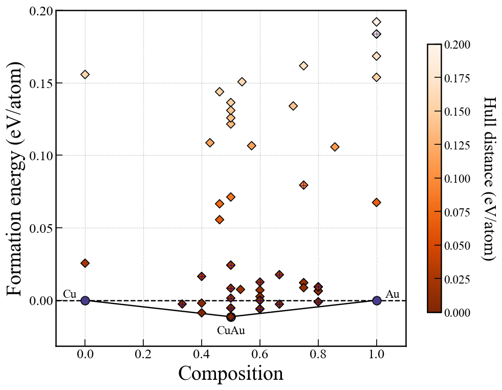
show_max：y軸上限（0.2）
label_stable：安定相の組成を表示するかどうか（True）
vmax：右のカラーバーの最大値（0.2）
bottom_margin：最小値とy軸下限の間のマージン（0.02）．
fig_format：図のファイルフォーマット．svg, png, pdfに対応．（svg）

マーカー上の十字の印は最新世代の探索結果を示している．

3元系

show_max：hull distanceがshow_max以下のものだけをプロット（0.2）
label_stable：安定相の組成を表示するかどうか（True）
vmax：右のカラーバーの最大値（0.2）
bottom_margin：3元系では無関係
fig_format：図のファイルフォーマット．svg, png, pdfに対応．（svg）

マーカーの十字の印は最新世代の探索結果を示している．

データのダウンロード

Jupyter notebook

先ほどダウンロードした結果の中にある data/ ディレクトリに移動する．その後，CrySPY utilityがローカルにダウンロードしてある場合は cryspy_analyzer_EA-vc.ipynb をコピーする．またはGitHubから直接ダウンロードしてくる（CrySPY_utility/notebook/）．

Jupyter notebookファイルには，CrySPYのコードと同じ関数が書かれており，自由に凸包のプロットをカスタマイズできる．適宜順番に実行していき，下記のどちらかを選ぶと自動プロットと同じものが得られる

Binary system, matplotlib
Ternary system, matplotlib

途中にある

Interactive plot using Plotly

では，2元系，3元系および4元系において，Plotlyを用いたインタラクティブプロットができる．プロット例はCrySPY > チュートリアル > インタラクティブモード（Jupyter Notebook） #Interactive plot using Plotlyを参考にすること．

Bayesian Optimization (BO)

LAQA

May 15th, 2023

情報

CrySPYの基本的な使い方に関してははじめにTutorial > Random Search (RS)を見ること．
ここではCrySPY 1.1.0以上を想定している．

ここで利用しているファイルはCrySPY_utility/examples/qe_Si16_LAQAからダウンロードできる．このチュートリアルでは，50個だけ初期構造を生成しているが，本来LAQAでは，もっと多くの構造を生成しておいてそこから良い候補を選択することでシミュレーションを進める．

Input

cryspy.in

cryspy.inの例．

[basic]
algo = LAQA
calc_code = QE
tot_struc = 50
nstage = 1
njob = 10
jobcmd = qsub
jobfile = job_cryspy

[structure]
atype = Si
nat = 16
mindist_1 = 1.5

[QE]
qe_infile = pwscf.in
qe_outfile = pwscf.out
kppvol =  80

[LAQA]
nselect_laqa = 4

[option]

LAQAではnstageは1にする必要がある．
[LAQA]セクションのnselect_laqaだけ新しく設定する必要がある． nselect_laqaは一回の選択で選ばれる候補の数．

下記のようにwfやwsを指定すれば，LAQAのスコアにおける重みも変えられる．省略した場合，デフォルトでは0.1と10.0がそれぞれ使われる．スコアの詳細についてはSearch algorithms > LAQAを見ること．

[LAQA]
nselect_laqa = 4
wf = 0.1
ws = 10.0

calc_in/pwscf.in_1

&control
    calculation = 'vc-relax'
    pseudo_dir = '/usr/local/gbrv/all_pbe_UPF_v1.5/'
    outdir='./outdir/'
    nstep = 10
/

&system
    ibrav = 0
    nat = 16
    ntyp = 1
    ecutwfc = 40
    ecutrho = 200
    occupations = 'smearing'
    degauss = 0.01
/

&electrons
/

&ions
/

&cell
/

ATOMIC_SPECIES
  Si -1.0 si_pbe_v1.uspp.F.UPF

nstepで1回の選択で何ステップ構造最適化を進めるかをコントロールする．(VASPではNSW)

calc_in/job_cryspy

#!/bin/sh
#$ -cwd
#$ -V -S /bin/bash
####$ -V -S /bin/zsh
#$ -N Si_CrySPY_ID
#$ -pe smp 20
####$ -q ibis1.q
####$ -q ibis2.q

mpirun -np $NSLOTS pw.x -nk 4 < pwscf.in > pwscf.out

if [ -e "CRASH" ]; then
    sed -i -e '3 s/^.*$/skip/' stat_job
    exit 1
fi

sed -i -e '3 s/^.*$/done/' stat_job

ジョブスクリプトはいつも使っているものと同じ

Run

ヒント

自動化スクリプトも用意してある．このページの最下部参照．

cryspyと打って1回目の実行．

cryspy &

この入力ファイルではまず50構造生成されるのでlog_cryspyを見て確認する．

2023/05/13 13:02:07
CrySPY 1.1.0
Start cryspy.py
Number of MPI processes: 1

Read input file, cryspy.in
Save input data in cryspy.stat

# --------- Generate initial structures
# ------ mindist
Si - Si 1.5
Structure ID      0 was generated. Space group: 165 --> 165 P-3c1
Structure ID      1 was generated. Space group:  66 -->  66 Cccm
Structure ID      2 was generated. Space group: 146 --> 146 R3
Structure ID      3 was generated. Space group:  82 -->  82 I-4
Structure ID      4 was generated. Space group: 162 --> 162 P-31m
...
...
...
Structure ID     47 was generated. Space group:  90 -->  90 P42_12
Structure ID     48 was generated. Space group: 214 --> 214 I4_132
Structure ID     49 was generated. Space group:  23 -->  23 I222

Elapsed time for structure generation: 0:00:10.929030


# ---------- Initialize LAQA
# ---------- Selection 0
selected_id: 50 IDs

LAQAでは，はじめに全ての初期構造の最適化ジョブを実行する．完全に最適化を終わらせるわけではなく，ここではnstep = 10にしているので，10ステップだけ実行される． cryspyコマンドを繰り返して，初期構造全てについて10ステップの最適化を完了させる．必要であれば，njobの値を上げておけば一度に多くのジョブがサブミットされる．

初めの最適化が全て終わると， log_cryspyの最後にLAQA is readyと表示される．

2023/05/13 13:23:31
CrySPY 1.1.0
Restart cryspy.py
Number of MPI processes: 1



# ---------- job status
ID     41: Stage 1 Done!

LAQA is ready

この状態でcryspy を実行すると，最初の選択が始まる．

2023/05/13 13:23:33
CrySPY 1.1.0
Restart cryspy.py
Number of MPI processes: 1



# ---------- job status

Backup data

# ---------- Selection 1
selected_id: 37 8 10 48

nselect_laqaで設定された構造の数だけ選択される． cryspyをもう一度実行するとそれらのジョブ（次の10ステップ）がサブミットされる．

cryspy &

2023/05/13 13:23:36
CrySPY 1.1.0
Restart cryspy.py
Number of MPI processes: 1



# ---------- job status
ID     37: submit job, Stage 1
ID      8: submit job, Stage 1
ID     10: submit job, Stage 1
ID     48: submit job, Stage 1

あとはこれを何度も繰り返し行うことでスコアに応じて選択された構造の最適化が10ステップずつ進行する．ある程度の構造の最適化が完全に完了するまで進めて，止めたいタイミングでストップする．

Status

シミュレーションの途中でスコアの確認がしたければ次のファイルを見ると良い：

./data/LAQA_status

他にもLAQAに関数ファイルがいくつか出力される：

./data_LAQA_bias
./data_LAQA_energy
./data_LAQA_score
./data_LAQA_selected_id
./data_LAQA_step

Analysis and visualization

ここではCrySPYのデータをローカルPCで解析する．スパコンやワークステーションで計算を行ったら，ローカルPCにデータをダウンロードしておく．今後必要なければ，ファイルサイズが大きいworkとbackupディレクトリは削除しておいて良い． pklデータはgzipしておくとファイルサイズを減らすことができる．

jupyter notebook

ダウンロードした結果のdata/ディレクトリに移動して，cryspy_analyzer_LAQA.ipynbをCrySPY utilityからコピーする．

このjupyter notebookを順番に実行していけば下記のようなグラフとgif画像が作成できる．この例では，アニメーションのために全ての構造の最適化を完全に完了させた．（全て最適化を完了させるとランダムサーチと計算量が変わらないのでLAQAの優位性はない）

このグラフはエネルギーを最適化ステップの関数として示している．赤い線は最終的にエネルギーが低かった3つの構造を表しており，中でも一番安定だった構造はダイアモンド構造に到達している．安定になる構造はかなり早い段階で選択されて構造最適化が完了していることがわかる．

情報

algo = LAQAでは[option]セクションの下記の二つは自動的にTrueになる．

force_step_flag = True
stress_step_flag = True

原子に働く力とストレスのデータは1ステップごとに収集される．エネルギーと構造データは1ステップごとではなく，選択ごとに収集される．つまり，この場合は10ステップおきにエネルギーと構造データは保存される．もし1ステップごとのデータが欲しいのであれば，手動で下記の設定を追加すること．

[option]
energy_step_flag = True
struc_step_flag = True

Auto script

何度も繰り返しcryspyを実行するのは面倒に感じたかもしれない．下記のようなスクリプトを使えば自動化できる．

repeat_cryspy

Molecular crystal structure prediction

情報

First, see Tutorial > Random Search (RS) for basic usage of CrySPY.

In this section, we give a tutorial on the molecular structure generation part only. Since version 0.9.0, CrySPY has been able to generate random molecular crystal structures using PyXtal.

You need to use a pre-defined molecular by PyXtal’s database (see, https://pyxtal.readthedocs.io/en/latest/Usage.html?highlight=benzene#pyxtal-molecule-pyxtal-molecule)) or create molecule files that define molecular structures.

Pre-defined molecule

PyXtal currently supports C60, H2O, CH4, NH3, benzene, naphthalene, anthracene, tetracene, pentacene, coumarin, resorcinol, benzamide, aspirin, ddt, lindane, glycine, glucose, and ROY.

Let us generate molecular crystal structures that consist of 2 benzenes.

Move to your working directory, and copy input example files by one of the following methods.

Download from CrySPY utility > examples > qe_benzene_2_RS_mol
Copy from CrySPY utility that you installed
(only version 0.10.3 or earlier) cp -r ~/CrySPY_root/CrySPY-0.9.0/example/QE_benzene_2_RS_mol .

Take a look at cryspy.in.

$ cat cryspy.in
[basic]
algo = RS
calc_code = QE
tot_struc = 6
nstage = 2
njob = 2
jobcmd = qsub
jobfile = job_cryspy

[structure]
struc_mode = mol
atype = H C
nat = 12 12
mol_file = benzene
nmol = 2

[QE]
qe_infile = pwscf.in
qe_outfile = pwscf.out
kppvol = 40  60

[option]

In generating molecular crystal structures, you have to set struc_mode = mol in the [structure] section. Molecule file(s) and the number of molecule(s) are specified as:

mol_file = benzene
nmol = 2

Run CrySPY and see the initial structures (./data/init_POSCARS).

User-defined molecule

Move to your working directory, and copy input example files for 2 formula units of Li3PS4.

version 1.0.0 or later
- Copy from CrySPY utility
version 0.10.3 or earlier
- cp -r ~/CrySPY_root/CrySPY-0.9.0/example/QE_Li3PS4_2fu_RS_mol .

$ cd QE_Li3PS4_2fu_RS_mol
$ ls
Li.xyz  PS4.xyz  calc_in/  cryspy.in

Molecule files of Li and PS4 are included. Supported formats in PyXtal are .xyz, .gjf, .g03, .g09, .com, .inp, .out, and pymatgen’s JSON serialized molecules.

$ cat Li.xyz
1
New structure
 Li  0.000  0.000  0.000

$ cat PS4.xyz
5
New structure
 P    0.000000    0.000000    0.000000
 S    1.200000    1.200000   -1.200000
 S    1.200000   -1.200000    1.200000
 S   -1.200000    1.200000    1.200000
 S   -1.200000   -1.200000   -1.200000

Check cryspy.in.

$ cat cryspy.in
[basic]
algo = RS
calc_code = QE
tot_struc = 4
nstage = 2
njob = 1
jobcmd = qsub
jobfile = job_cryspy

[structure]
struc_mode = mol
atype = Li P S
nat = 6 2 8
mol_file = ./Li.xyz  ./PS4.xyz
nmol = 6 2

[QE]
qe_infile = pwscf.in
qe_outfile = pwscf.out
kppvol = 40  60

[option]

A single atom (Li atom in this case) is treated as a molecule in the molecular crystal structure generation mode. In this example, a random molecular structure is composed of six Li molecules (atoms) and two PS4 molecules specified as:

mol_file = ./Li.xyz ./PS4.xyz
nmol = 6 2

In mol_file, set relative path of molecule files from cryspy.in. Here the molecule files are placed in the same directory.

Run CrySPY and see the initial structures (./data/init_POSCARS).

timeout_mol

Molecular crystal structure generation can be time consuming because PyXtal calculates the molecule directions according to a specified space group. Sometimes molecular crystal structure generation gets stuck. So we set a time limit on the single structure generation. The time limit (timeout_mol) is set to 120 seconds by default. If the limit is insufficient, you have to increase it as (see last line):

struc_mode = mol
atype = Li P S
nat = 6 2 8
mol_file = ./Li.xyz  ./PS4.xyz
nmol = 6 2
timeout_mol = 300.0

Volume of unit cell

You can control the volume of unit cells by changing the value(s) of scaling factor, vol_factor, in cryspy.in. By default, vol_factor is set to 1.0. It is also possible to specify a range of factors. Set minimum and maximum values as follows:

struc_mode = mol
atype = Li P S
nat = 6 2 8
mol_file = ./Li.xyz  ./PS4.xyz
nmol = 6 2
timeout_mol = 300.0
vol_factor = 0.8 1.5

Random structure generation with MPI

2023/10/21 update

情報

CrySPYの基本的な使い方に関してはチュートリアル > Random Search (RS)を見ること．

情報

動作環境:

CrySPY ~~1.1.0~~ 1.2.3 or later
mpi4py
MPI library (Open MPI, Intel MPI, MPICH, etc.)

警告

1.1.0 <= CrySPY <=1.2.2ではバグがあった． MPIを使ったジョブをbashやzshで実行するとき（e.g., jobcmd = zsh, jobfile = job_cryspy），MPIのジョブが流れない． qsubやsbatchでジョブスケジューラーを使う場合は問題ない。このバグはバージョン1.2.3で修正．

mpi4py

mpi4pyのインストールがまだであればインストールする．

pip install mpi4py

入力ファイル

cryspy.inはいつもと同じで変更する必要はない．ここでは下記の設定でMPIを使った構造生成を行う．

[basic]
algo = RS
calc_code = soiap
tot_struc = 100
nstage = 1
njob = 2
jobcmd = zsh
jobfile = job_cryspy

[structure]
atype = Si
nat = 8

[soiap]
soiap_infile = soiap.in
soiap_outfile = soiap.out
soiap_cif = initial.cif

[option]

tot_struc，atype，nat以外の変数は構造生成に関係がないのでここでは無視して良い．

実行

4並列で実行する場合，mpiexec -nを使う．-pオプションも必要．

mpiexec -n 4 cryspy -p

In 1.1.0 <= CrySPY <= 1.2.2では下記のコマンド (-pオプションは使用しない)

mpiexec -n 4 cryspy

ジョブスケジューラーなどにサブミットするときは自分でジョブファイルを作る．下記は一例．

#!/bin/sh
#$ -cwd
#$ -V -S /bin/bash
#$ -N n_nproc
#$ -pe smp 4

mpirun -np $NSLOTS ~/.local/bin/cryspy

実行スクリプトcryspyのpathなどは適宜編集すること．

結果

CrySPYはシンプルに構造生成タスクをプロセス数で分割している．

Rank 0: IDs 0 – 24
Rank 1: IDs 25 – 49
Rank 2: IDs 50 – 74
Rank 3: IDs 75 – 99

構造が生成された順番でログが出力される．

2023/04/24 22:47:51
CrySPY 1.1.0
Start cryspy.py
Number of MPI processes: 4

Read input file, cryspy.in
Save input data in cryspy.stat

# --------- Generate initial structures
# ------ mindist
Si - Si 1.11
Structure ID     25 was generated. Space group: 138 --> 123 P4/mmm
Structure ID     75 was generated. Space group:  99 -->  99 P4mm
Structure ID      0 was generated. Space group: 127 --> 123 P4/mmm
Structure ID      1 was generated. Space group:  61 -->  61 Pbca
Structure ID     50 was generated. Space group:  38 -->  38 Amm2
Structure ID     51 was generated. Space group: 134 --> 123 P4/mmm
Structure ID     26 was generated. Space group: 111 --> 123 P4/mmm
Structure ID      2 was generated. Space group:   9 -->   9 Cc
Structure ID      3 was generated. Space group:  80 -->  80 I4_1
Structure ID      4 was generated. Space group: 107 --> 107 I4mm
Structure ID      5 was generated. Space group:  75 -->  75 P4
Structure ID     76 was generated. Space group: 108 --> 108 I4cm
Structure ID     77 was generated. Space group: 100 --> 100 P4bm
Structure ID     27 was generated. Space group: 207 --> 221 Pm-3m

しかし，init_POSCARSでは，構造生成が全て終わった後に出力しているのでID順になっている．

ID_0
1.0
   2.9636956737951818    0.0000000000000002    0.0000000000000002
   0.0000000000000000    2.9636956737951818    0.0000000000000002
   0.0000000000000000    0.0000000000000000    6.2634106638053080
Si
8
direct
  -0.1602734164607877   -0.1602734164607877   -0.0000000000000000 Si
   0.1602734164607877    0.1602734164607877    0.5000000000000000 Si
   0.6602734164607877    0.3397265835392123    0.7500000000000000 Si
   0.3397265835392122    0.6602734164607877    0.2500000000000000 Si
   0.4469739273741755    0.4469739273741755   -0.0000000000000000 Si
   0.5530260726258245    0.5530260726258244    0.5000000000000000 Si
   0.0530260726258245    0.9469739273741754    0.7500000000000000 Si
   0.9469739273741754    0.0530260726258245    0.2500000000000000 Si
ID_1
1.0
   7.2751506682509657    0.0000000000000004    0.0000000000000004
   0.0000000000000000    7.2751506682509657    0.0000000000000004
   0.0000000000000000    0.0000000000000000    5.1777634169924873
Si
8
direct
  -0.3845341807505553   -0.3845341807505553    0.4999999999999999 Si
   0.3845341807505553    0.3845341807505553    0.5000000000000000 Si
   0.3845341807505553   -0.3845341807505553    0.0000000000000000 Si
  -0.3845341807505553    0.3845341807505553   -0.0000000000000000 Si
   0.0000000000000000    0.5000000000000000    0.2500000000000000 Si
   0.5000000000000000    0.0000000000000000    0.7500000000000000 Si
   0.0000000000000000    0.5000000000000000    0.7500000000000000 Si
   0.5000000000000000    0.0000000000000000    0.2500000000000000 Si
ID_2
1.0
  -4.3660398676292269   -4.3660398676292269    0.0000000000000000
  -4.3660398676292269   -0.0000000000000003   -4.3660398676292269
   0.0000000000000000   -4.3660398676292269   -4.3660398676292269
Si
8
direct
   0.8700001548800920    0.8700001548800920    0.1299998451199080 Si
   0.1299998451199080    0.1299998451199080    0.8700001548800920 Si
   0.8700001548800920    0.1299998451199080    0.8700001548800920 Si
   0.1299998451199080    0.8700001548800920    0.1299998451199080 Si
   0.1299998451199080    0.8700001548800920    0.8700001548800920 Si
   0.8700001548800920    0.1299998451199080    0.1299998451199080 Si
   0.7500000000000000    0.7500000000000000    0.7500000000000000 Si
   0.2500000000000000    0.2500000000000000    0.2500000000000000 Si

メモ

ランダム構造生成以外の部分はMPIを使っても並列化されていないので意味はない．

情報

インタラクティブモード (Jupyter Notebook)

2025年3月6日

情報

動作環境:

CrySPY 1.4.0以上
Jupyter
ASE対応の構造最適化計算ソフト（汎用機械学習ポテンシャルなど）
nglview (optional)

準備

CrySPYをインストールすればASEは自動的にインストールされている．ワークステーションやローカルPCでJupyterを使えるようにしておく．このチュートリアルでは，構造最適化にPure Python EMT calculatorを用いる．このEMTポテンシャルの精度は悪く，デモ用のものなので注意．

exampleのノートブックには汎用機械学習ポテンシャルのCHGNetを使用するコードも書いてあるので，CHGNetを試したい場合は事前にpipでインストールしておく．

入力ファイル

どこか適当なワーキングディレクトリに移動して，まずはexampleをコピーしてくる．下記のどちらからコピーしてきても良い．

CrySPY_utility/examples/interactiveからダウンロード
インストールしておいたCrySPY utilityからコピーする

インタラクティブモードでも，cryspy.inを入力ファイルとして使用する．インタラクティブモードではcalc_inディレクトリは使用しない． input_examplesディレクトリの中に，いくつかの入力ファイル例が入っているので参考にしてほしい．

ここではEA-vcを用いた下記のcryspy.inを使用する．EA-vcについてはEA-vcのチュートリアルを見ること．

[basic]
algo = EA-vc
calc_code = ASE
nstage = 1
njob = 10
jobcmd = zsh
jobfile = job_cryspy

[structure]
atype = Cu Au
ll_nat = 0 0
ul_nat = 8 8

[ASE]
ase_python = ase_in.py

[EA]
n_pop = 20
n_crsov = 5
n_perm = 2
n_strain = 2
n_rand = 2
n_add = 3
n_elim = 3
n_subs = 3
target = random
n_elite = 2
n_fittest = 10
slct_func = TNM
t_size = 2
maxgen_ea = 5
end_point = 0.0 0.0

[option]

ノートブック

cryspy_interactive.ipynbを開いて，上から実行していく．

Check current working directory

最初のセルはファイルやcryspy.inの中身を確認しているだけ．

!pwd
print()
!ls
print()
!cat cryspy.in

Import

コメントアウトされているものは今回は無視して，CrySPYのインタラクティブモードで核となるライブラリをインポートするセルを実行する．

# ---------- import
from cryspy.interactive import action

Initialize CrySPY

このセルは通常の初回実行に対応している．cryspy.inを読み込んで初期構造が生成される．

# ---------- initial structure generation
action.initialize()

Set calculator

このセルでASEのcalculatorをセットする．ここではASEのEMTを用いる．

# ---------- EMT in ASE
from ase.calculators.emt import EMT
calculator = EMT()

# ---------- CHGNet
#from chgnet.model import CHGNetCalculator
#calculator = CHGNetCalculator()

Restart CrySPY

このセルを実行すると，先ほど生成した初期構造の最適化が始まる．インタラクティブモードでは一つ一つ順番に構造最適化計算を行う．その際に進捗バーも表示される．

# ---------- structure optimization
action.restart(
    njob=20,    # njob=0: njob in cryspy.in will be used
    calculator=calculator,
    optimizer='BFGS',    # 'FIRE', 'BFGS' or 'LBFGS'
    symmetry=True,       # default: True
    fmax=0.01,           # default: 0.01 eV/Å
    steps=2000,          # default: 2000
)

njob: 一度の実行で最適化計算を行う構造数．0の場合はcryspy.inに書いてある値が使用される．
calculator: 先に設定したcalculatorを代入
optimizer: FIRE, BFGS, LBFGSから選択．文字列で指定する．
symmetry: Trueなら対称性を維持した構造最適化を行う
fmax: 収束判定に使われる原子に働く力の最大値（eV/Å）
steps: 最大最適化ステップ数

njobの値を小さくしている場合は，何度かこのセルを実行して，全ての初期構造の最適化を終了させる． EA-vcを用いている場合，すべて終わると以下のように表示される．

EA is ready

もう一度このセルを実行すると世代交代が行われるので，次世代の構造生成が終了したら，あとは同様にこのセルの実行を繰り返す．

Show results

このセルを実行すると，cryspy_rslt_energy_ascなどのファイルを表示できる．

# ---------- show results
#!cat ./data/cryspy_rslt    # Order of structure optimization completion
!cat ./data/cryspy_rslt_energy_asc    # show energy ascending order
#!sed -n 2,4p ./data/cryspy_rslt    # show i--jth lines
#!tail -n 5 ./data/cryspy_rslt    # show last 5 lines

Structure visualization

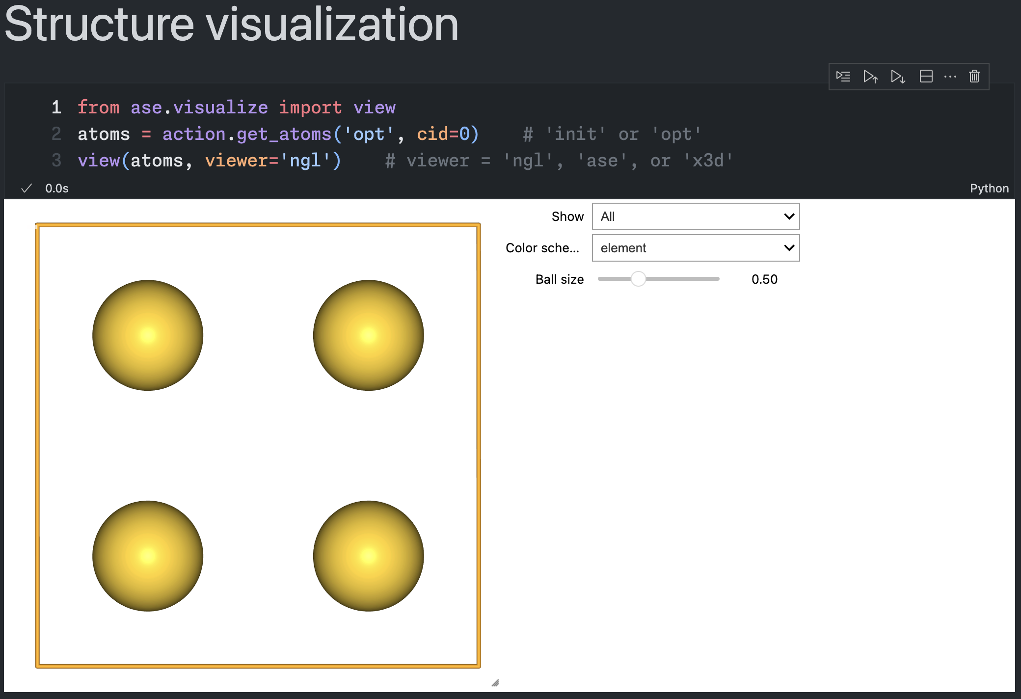
初期構造や最適化済みの構造をインタラクティブに可視化できる．

from ase.visualize import view
atoms = action.get_atoms('opt', cid=0)    # 'init' or 'opt'
view(atoms, viewer='ngl')    # viewer = 'ngl', 'ase', or 'x3d'

action.get_atoms('opt', cid=0)のところでoptをinitに変えると，初期構造が確認できる． cidで構造IDを指定する． ASEの機能を使用しているのでviewerにはngl, ase, x3dが利用できる． nglを使うにはnglviewのインストールが必要なのでpipでインストールしておく．

Energy plot for RS, EA

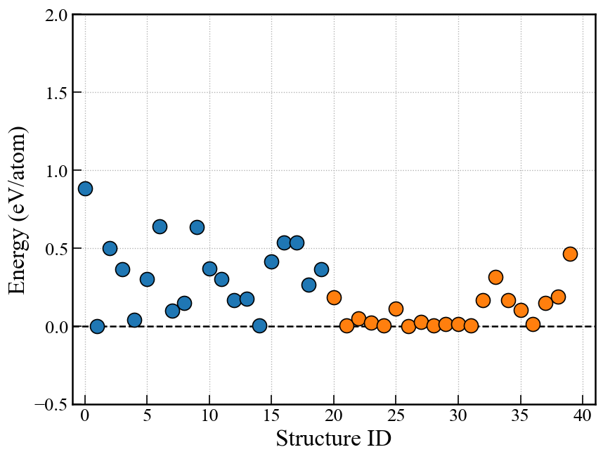
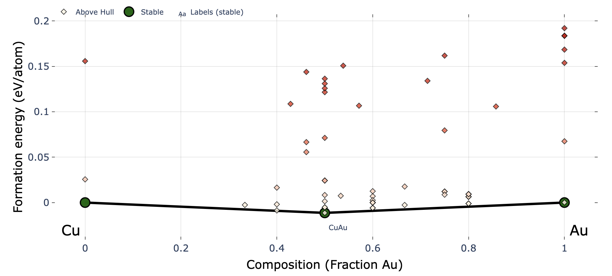
ランダムサーチ（RS）や進化的アルゴリズム（EA）の場合，下記画像のようなエネルギーグラフを表示できる． EA-vcの場合は原子数が異なるので単純にエネルギーを比較できないので，後述のconvex hullプロットを使う．

fig, ax = action.plot_E(
              title=None,
              ymax=2.0,
              ymin=-0.5,
              markersize=12,
              marker_edge_width=1.0,
              marker_edge_color='black',
              alpha=1.0,
          )

Convex hull plot for EA-vc

Interactive plot using Plotly

EA-vcの場合はPlotlyを用いたconvex hullのインタラクティブプロットが利用できる． CrySPYをインストールすればPlotlyは自動的にインストールされている．このconvex hullプロットはpymatgenの機能を用いている．

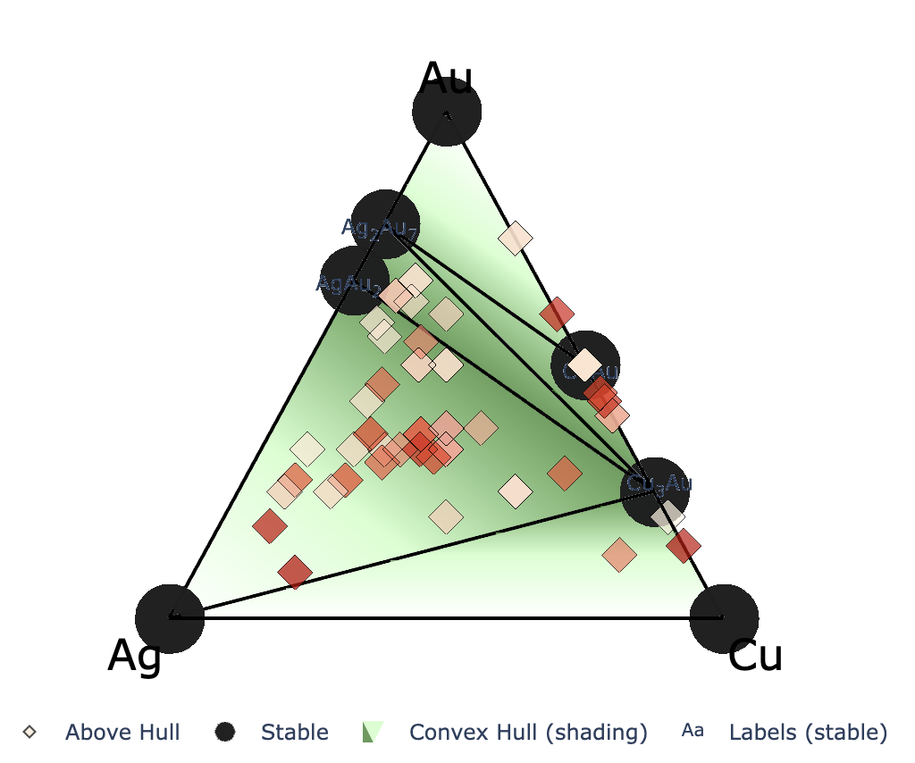
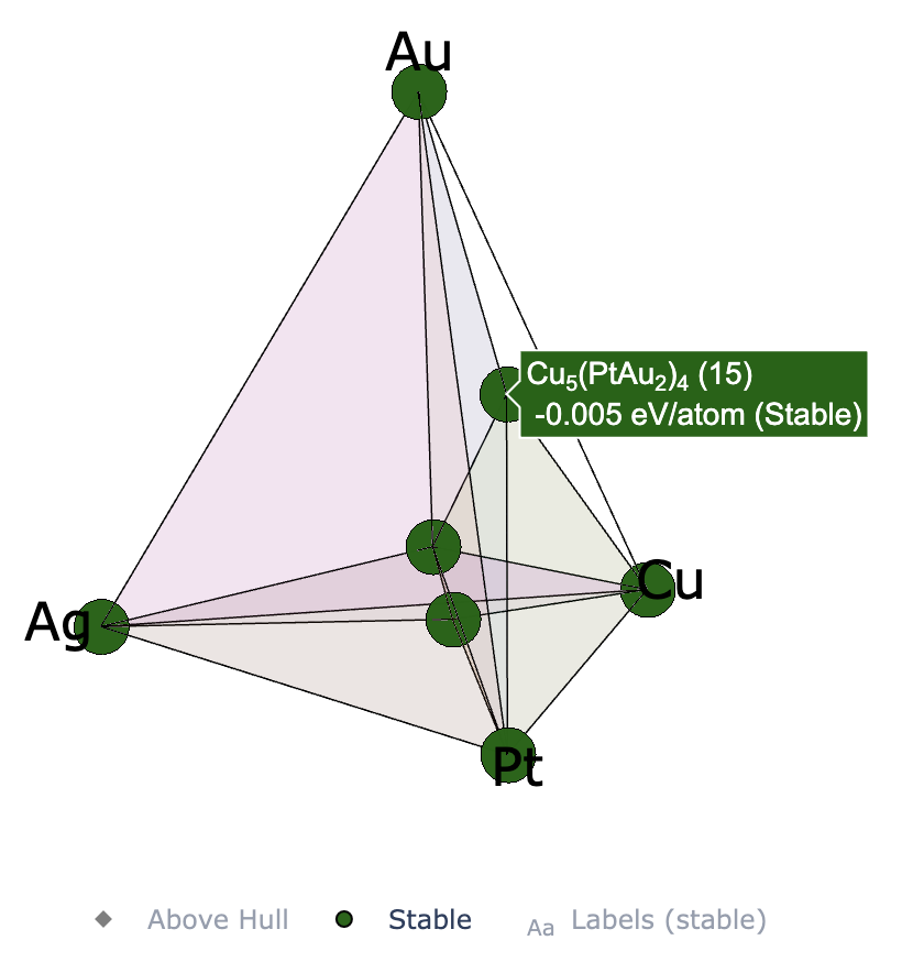
action.interactive_plot_convex_hull(cgen=None, show_unstable=0.2, ternary_style='2d')

cgen: どの世代までプロットするかを指定．Noneであれば最新の世代までプロットされる．
show_unstable: 描画するhull distanceの最大値．
ternary_style
- 2元系: ternary_style = ‘2d’
- 3元系: ternary_style = ‘2d’, ‘3d’
- 4元系: ternary_style = ‘3d’

2元系ではなく，3元系や4元系で計算しているときは下記のようなインタラクティブプロットが得られる．左から順に，3元系（ternary_style = ‘2d’），3元系（ternary_style = ‘3d’），4元系（ternary_style = ‘3d’）のプロット

Binary system using matplotlib

このセルを実行すると，matplotlibを用いて2元系のconvex hullをプロットできる．

fig, ax = action.plot_convex_hull_binary(
              cgen=None,
              show_max=0.2,
              label_stable=True,
              vmax=0.2,
              bottom_margin=0.02,
          )
fig    # to show plot in jupyter

cgen: どの世代までプロットするかを指定．Noneであれば最新の世代までプロットされる．
show_max: 描画するhull distanceの最大値．
label_stable: 安定相のラベルを表示するかどうか．
vmax: カラーバーのhull distaceの最大値．
bottom_margin: y軸の下部のマージン．

Ternary system using matplotlib

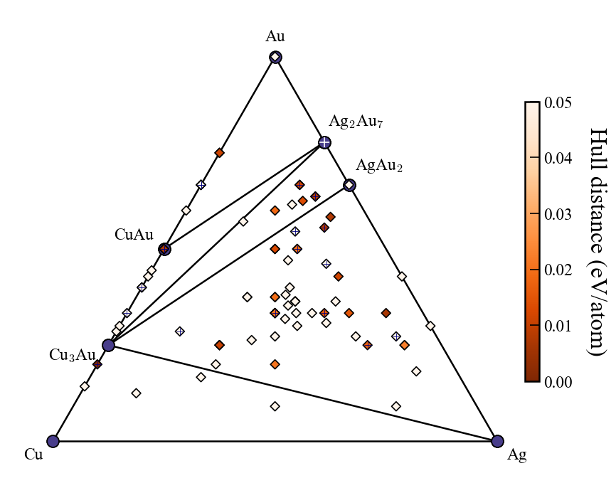
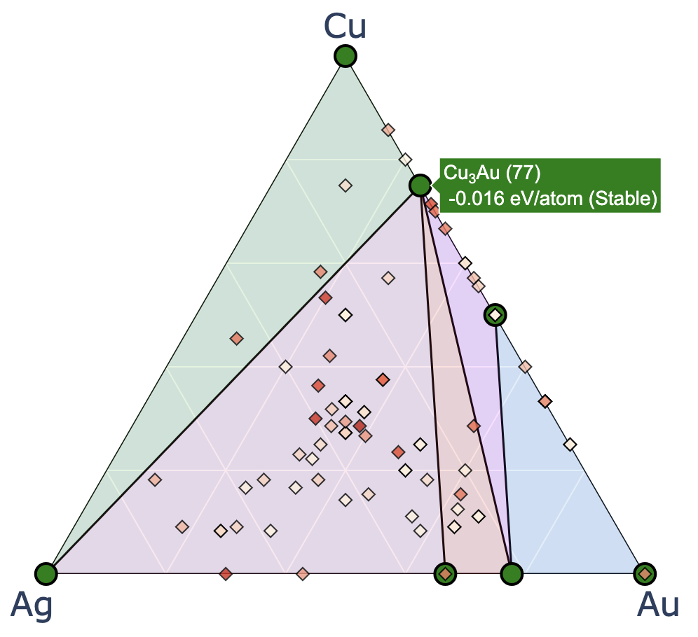
もし3元系の探索をしている場合は，このセルを実行することでmatplotlibを使ったconvex hullのプロットができる．

fig, ax = action.plot_convex_hull_ternary(
              cgen=None,
              show_max=0.2,
              label_stable=True,
              vmax=0.2,
          )
fig    # to show plot in jupyter

cgen: どの世代までプロットするかを指定．Noneであれば最新の世代までプロットされる．
show_max: 描画するhull distanceの最大値．
label_stable: 安定相のラベルを表示するかどうか．
vmax: カラーバーのhull distaceの最大値．

例えば以下のようなプロットが得られる．

チュートリアル

目次

チュートリアルのサブセクション

ランダムサーチ (RS)

入力ファイルの準備

CrySPY実行

ランダムサーチ (RS)のサブセクション

ASE on your local PC

Assumption

Input files

cryspy.in

calc_in directory

Job file

Input for ASE

CrySPY実行

soiap on your local PC

Assumption

Input files

cryspy.in

calc_in directory

Job file

Input for soiap

CrySPY実行

VASP

Assumption

Input files

cryspy.in

calc_in directory

Job file

Input for VASP

CrySPY実行

QE

Assumption

Input files

cryspy.in

calc_in directory

Job file

Input for QE

CrySPY実行

OpenMX

LAMMPS

Check cryspy.in

[basic] section

[structure] section

Script to run

Assumption

Make script

Firsrt run

Submit job

計算再開

ジョブの投入

Check results

Append structures

解析と可視化

データのダウンロード

Jupyter notebook

進化的アルゴリズム（EA）

入力ファイルの準備

CrySPY実行

進化的アルゴリズム（EA）のサブセクション

ASE on your local PC

cryspy.in

calc_in/

calc_in/ase_in.py

calc_in/job_cryspy

次世代の生成

初回実行

構造最適化

次世代生成

結果の確認

cryspy_rslt

ea_info

ea_origin

解析と可視化

データのダウンロード

Jupyter notebook

組成可変型進化的アルゴリズム（EA-vc）

入力ファイルの準備

CrySPY実行

組成可変型進化的アルゴリズム（EA-vc）のサブセクション