Subsections of Search algorithms
Random search (RS)
under construction
Evolutionary algorithm (EA)
2025 April 2
Background
Evolutionary algorithms (EAs) are metaheuristic methods inspired by the theory of evolution. EA can effectively generate new structures (offspring) by inheriting the local environments of the stable structures (parents) explored so far. Oganov group’s USPEX is a well-known software, and there are others such as XtalOpt. For example, there are previous studies such as the following papers.
- T. S. Bush, C. R. A. Catlow, and P. D. Battle, J. Mater. Chem. 5, 1269 (1995).
- A. R. Oganov and C. W. Glass, J. Chem. Phys. 124, 244704 (2006).
- A. R. Oganov, A. O. Lyakhov, and M. Valle, Acc. Chem. Res. 44, 227 (2011).
- A. O. Lyakhov, A. R. Oganov, H. T. Stokes, and Q. Zhu, Comput. Phys. Commun. 184, 1172 (2013).

Procedure
- Initialize population
- Evaluate fitness
- Natural selection
- Select parents
- Create next generation
- Repeat from step 2: Evaluate fitness
Initialize population
In the first generation, a set of random structures is generated according to the number specified by n_pop.
tot_struc is not used in EA or EA-vc.
Evaluate fitness
Currently, energy is the only property that can be used as fitness in CrySPY.
By setting fit_reverse = False, the algorithm is configured to search for the minimum value.
The fit_reverse setting is designed for future cases where fitness may be based on properties other than energy.
Natural selection
DFT calculations occasionally fail and produce extremely unreasonable energy values.
emax_ea and emin_ea can be used to filter out structures with unreasonably low (or high) energy values:
$$ \mathrm{emin\_ea} \le E \ (\mathrm{eV/atom}) \le \mathrm{emax\_ea} $$
For example, if emin_ea is set, any structure with an energy lower than that value will be ignored.
In natural selection, the current population and elite individuals preserved from previous generations are first ranked based on fitness.
The number of elite individuals used here is specified by n_elite.
Only the top n_fittest individuals among the current population and elite individuals are selected, while all others are eliminated.
During the natural selection process, duplicates are removed using the StructureMatcher class provided by pymatgen, and then the top n_fittest individuals are selected.
n_fittest is often set to about half of n_pop (the population size).
Note that in the current implementation, if n_fittest = 0, all individuals are retained.
The figure below shows an example of the natural selection process when n_fittest = 5.

Select parents
Two parent selection methods are implemented in CrySPY to select a single parent individual from the candidate parents.
Both methods are designed so that individuals with higher fitness have a higher probability of being selected.
Setting slct_func = TNM enables tournament selection, while slct_func = RLT enables roulette selection.
Tournament selection requires fewer parameters and is easier to use.
Create next generation
The next generation consists of offspring produced by evolutionary operations on candidate parents, along with some randomly generated structures. Random structures are added in each generation to maintain diversity and to help escape from local minima.
Evolutionary operations
Here, we introduce the operations of the fixed-composition EA implemented in CrySPY.
Population size
The sum of structures from crossover, permutation, strain, and random generation must be equal to n_pop.
n_pop=n_crsov+n_perm+n_strain+n_rand
Subsections of Evolutionary algorithm (EA)
Crossover
Overview
Crossover is an evolutionary operation that creates a new structure (offspring) by exchanging sliced regions between two parent structures. This promotes structural diversity and enables the inheritance of locally stable features. It is one of the main operators used to explore low-energy configurations in structure search.
How it works
- Select two distinct individuals from the candidate parents
- Perform a random translation
- Randomly select a lattice vector
- Slice the parents near the center
- Swap the sliced halves
- Select the offspring with more atoms
- Adjust the number of atoms near the border
- Perform a minimum interatomic distance check

4. Slice the parents near the center
The slice point is placed near the center and slightly varied each time.
slice_point = np.clip(np.random.normal(loc=0.5, scale=0.1), 0.3, 0.7)
If any of the subsequent steps fail, the process may be restarted from step 4.
However, the number of retries is limited to maxcnt_ea, and if this limit is exceeded, the parent selection step is repeated.
5. Swap the sliced halves
When crs_lat is set to random, the lattice vectors of one of the two parent structures are randomly selected.
When crs_lat is set to equal, the average of the lattice vectors of the two parent structures is used.
The default is random.
6. Select the offspring with more atoms
Swapping the sliced parts of the parent structures results in two structures with different numbers of atoms. Temporarily, we select the structure with more atoms.

However, if the composition differs too much from the target, the process restarts from step 4 (Slice the parents near the center).
The tolerance for the difference in the number of atoms is set by nat_diff_tole.
The default value of nat_diff_tole is 4, which allows a tolerance of ±4 atoms per element.
In the figure above, the number of blue atoms is -1 and the number of green atoms is +2 relative to the original composition.
7. Adjust the number of atoms near the border
Deletion
When adjusting the number of atoms, the process starts with atom deletion.
The number of green atoms is excessive and needs to be reduced.
As illustrated in the figure below, atoms that do not satisfy the minimum interatomic distance defined by mindist are preferentially removed.

As shown below, if atoms that violate the minimum interatomic distance remain after the deletion process, the procedure is restarted from step 4 (Slice the parents near the center).

If there are no atoms violating the minimum interatomic distance but atoms still need to be deleted, atoms are removed in order of increasing distance from the border, as shown in the figure below. Note that, in addition to the central slicing point, positions with internal coordinates of 0 are also considered borders.

Addition
When atoms are lacking, the missing atoms are added near the border. The internal coordinate along the selected axis is determined as shown below. Here, mean refers to either the slice point or 0.
coords[axis] = np.random.normal(loc=mean, scale=0.08)
The remaining two components of the coordinate are determined randomly. Atoms are added until the target number is reached, while checking for violations of the minimum interatomic distance.

Permutation
Overview
Permutation is an evolutionary operation that generates new structures (offspring) by modifying the atomic arrangement within a single structure. It enables the exploration of alternative configurations without changing the lattice or the overall composition.
How it works
The positions of atoms of different elements are swapped.
The number of swaps can be specified by ntimes, which is set to 1 by default.
After the swap, a minimum interatomic distance check is performed.

Strain
Overview
Strain is an evolutionary operation that generates a new structure (offspring) by applying a small random distortion to the lattice of a parent structure. It helps to explore nearby regions of the configuration space while preserving atomic connectivity and composition. This operator is useful for fine-tuning structural candidates and escaping local minima.
How it works
The lattice vectors are $ \mathbf{a} $ transformed to $ \mathbf{a}' $ by applying a strain matrix, as follows:
$$ \mathbf{a}' = \begin{pmatrix} 1 + \eta_1 & \frac{1}{2} \eta_6 & \frac{1}{2} \eta_5 \\ \frac{1}{2} \eta_6 & 1 + \eta_2 & \frac{1}{2} \eta_4 \\ \frac{1}{2} \eta_5 & \frac{1}{2} \eta_4 & 1 + \eta_3 \end{pmatrix} \mathbf{a}. $$Here,
$ \eta_i $ are given by a Gaussinan distribution
$ \mathcal{N}\left( 0, \ \sigma_{\mathrm{st}}^2 \right) $.
$ \sigma_{\mathrm{st}} $ is specified by the input parameter sigma_st (by default, sigma_st = 0.5).
As shown in the figure below, the lattice is deformed and then rescaled to restore the original volume.
Finally, the minimum interatomic distance constraint is checked.

Tournament selection
Overview
Tournament selection is a method used to choose parent individuals from the candidate parents based on their fitness.
It is designed to balance selection pressure and diversity in the population.
The figure below shows an example with n_fittest = 10 and t_size = 3.

How it works
- A fixed number of individuals (
t_size) are randomly selected from the candidate parents. - Among them, the individual with the highest fitness (i.e., lowest energy) is chosen as the parent.
- This process is repeated until the required number of parents is selected.
Advantages
- Simple and efficient
- Requires only one parameter (
t_size) - Can control selection pressure by adjusting
t_size
Notes
- The default value of
t_sizeis 3. - If
t_sizeis small, diversity is promoted. - If
t_sizeis large, selection pressure increases, favoring the fittest individuals. - Unlike roulette selection, tournament selection never chooses the bottom (
t_size- 1 ) individuals from the candidate parents.
Roulette selection
Overview
Roulette selection is a probabilistic method used to select parent individuals from the candidate parents based on their fitness. In roulette selection, each individual’s chance of being selected is proportional to its fitness.
How it works
- When
fit_reverseis set toFalse(default), corresponding to minimization mode where energy is used as fitness, the fitness values of the candidate parents are multiplied by –1. - The fitness values
$ f_i $ are linearly scaled into
$ f'_i $ using the following equation, where
$ a $ and
$ b $ are parameters specified by
a_rltandb_rlt, respectively (with the condition that $ a > b $). $$ f_i' = \frac{a - b}{f_{\mathrm{max}} - f_{\mathrm{min}}} f_i + \frac{b f_{\mathrm{max}} - a f_{\mathrm{min}}}{f_{\mathrm{max}} - f_{\mathrm{min}}} $$ - The scaled fitness values $ f_i’ $ are converted into selection probabilities using the following equation: $$ p_i = \frac{f_i’}{\sum_k f_k’} $$ Each probability $ p_i $ represents the likelihood of selecting the $ i $-th individual.
- Parent individuals are then selected one by one according to the probabilities $ p_i $ using roulette wheel sampling, until the required number of parents is obtained.
Advantages
- All individuals have a non-zero chance of being selected
- Selection pressure can be adjusted by scaling the fitness values
Notes
- By default,
a_rlt = 10.0andb_rlt = 1.0 - Proper scaling of fitness values is important to ensure meaningful selection pressure.The figure below shows examples of $ p_i $ when $ a $ is relatively small (left) and relatively large (right). If $ a $ is too small, the selection pressure becomes weak, making it more difficult to favor individuals with higher fitness.

Variable-composition evolutionary algorithm (EA-vc)
2025 July 7, updated
Overview
Since CrySPY 1.4.0, a variable-composition EA (EA-vc) has been available as an extension of the fixed-composition EA. Refer to the following page for the supported interfaces (Interface). Although the overall flow is similar to the fixed-composition EA, EA-vc differs in how fitness is evaluated and how offspring are generated in order to handle varying compositions. Here, we describe the parts that have been modified from the original EA.
From version 1.4.1, it is possible to generate structures under the charge neutrality condition.
Procedure
- Initialize population
- Evaluate fitness
- Natural selection
- Select parents
- Create next generation
- Repeat from step 2: Evaluate fitness
Initialize population
In the first generation, a set of random structures is generated according to the number specified by n_pop.
tot_struc is not used in EA or EA-vc.
In EA-vc, the number of atoms for each atom type is randomly determined within a user-defined range.
The minimum (ll_nat) and maximum (ul_nat) number of atoms per type can be specified in cryspy.in as shown below.
[structure]
atype = Cu Au
ll_nat = 0 0
ul_nat = 8 8
Evaluate fitness
The convex hull computed from formation energies is used to evaluate the phase stability of different compositions, since directly comparing total energies of structures with different numbers of atoms is not meaningful. Information on formation energy, the convex hull, and phase diagrams can be found online. For example, see Materials Project Documentation. In EA-vc, the fitness is defined as the energy above hull (also referred to as hull distance).

Formation energy
Formation energy is calculated based on the reference energies (in eV/atom) of stable pure elements, which are specified as end_point in cryspy.in.
For example, in the case of the Cu–Au binary system, the end_point should contain the per-atom energies (in eV/atom) of fcc-Cu and fcc-Au, in that order.
Note that even if a structure with the same composition as end_point is found during the structure search and has a total energy lower than the corresponding end_point value, the formation energy is still currently calculated based on the original end_point values defined in cryspy.in.
Convex hull
The energy difference between a given structure’s formation energy and the convex hull is called the energy above hull, also known as the hull distance. This value indicates how much higher the formation energy of a structure is compared to the most stable combination of phases at the same composition. Structures with a hull distance of zero are on the convex hull and are thus thermodynamically stable.
Unlike in the fixed-composition EA, EA-vc filters structures based on their per-atom energy when computing the convex hull, using the condition: $$ \mathrm{emin\_ea} \le E \le \mathrm{emax\_ea} $$ Note that this filtering is based only on the total energy per atom, not on the formation energy.
To compute the convex hull, CrySPY uses the PhaseDiagram class provided by the pymatgen library.
Unlike in the case of formation energy, if a structure with the same composition as a pure element has a total energy lower than the corresponding end_point value, that structure is used as the reference for computing the convex hull and hull distance.
Natural selection
As shown in the figure below, EA-vc can produce multiple stable structures (i.e., with a hull distance of 0).
In such cases, multiple individuals share the top rank in terms of hull distance.
If the number of elite structures specified by n_elite is smaller than the number of equally ranked individuals, the selection becomes non-deterministic.
Currently, CrySPY randomly selects n_elite individuals from those with a hull distance less than 0.001 eV/atom.
If the number of individuals with a hull distance less than 0.001 eV/atom is smaller than n_elite, elite structures are selected in the usual way, based on fitness ranking.
When selecting elite individuals as well, duplicate structures are removed using the StructureMatcher class provided by the pymatgen library.

Elite individuals are selected based on the best structures from previous generations. However, because hull distance can vary from one generation to the next, the values for elite individuals are recalculated using the current convex hull before natural selection is applied.
As described in the Convex hull section, emin_ea and emax_ea are not used for natural selection in EA-vc.
Select parents
The method for selecting parents is the same as in the fixed-composition EA.
Create next generation
Evolutionary operations
The crossover (vc) operation is slightly different from that in the fixed-composition EA, while permutation and strain are the same. EA-vc introduces several new operations to enable compositional variation.
Population size
The sum of structures from crossover, permutation, strain, addition, elimination, substitution, and random generation must be equal to n_pop.
n_pop=n_crsov+n_perm+n_strain+n_add+n_elim+n_subs+n_rand
Subsections of Variable-composition evolutionary algorithm (EA-vc)
Crossover (vc)
The variable-composition crossover is almost the same as the fixed-composition version, but it differs in that the adjustment of the number of atoms is minimized.
In step 6 of the fixed-composition crossover, the difference in the number of atoms in each atom type is calculated directly.
In contrast, in crossover (vc), the difference is calculated based on the allowed range defined by ll_nat and ul_nat.
For example:
ll_nat = [4, 4, 4]
ul_nat = [8, 8, 8]
offspring_nat = [2, 6, 12]
nat_diff = [-2, 0, 4]
If this difference in the number of atoms (nat_diff in the example above) exceeds the allowed tolerance (nat_diff_tole), the operation is retried.
Otherwise, the number of atoms is adjusted to fall within the range defined by ll_nat and ul_nat.
Addition
2025 July 7, updated
An atom type whose current count does not exceed the limit specified by ul_nat is randomly selected, and one atom of that type is added at a random position.
From version 1.4.1, the functionality to add multiple atoms has been implemented. The number of atoms to be added is randomly selected from natural numbers up to add_max.
The default value is add_max = 3.
- Add one atom and check whether it satisfies the minimum interatomic distance specified by
mindist. - If the distance condition is not satisfied, the atom is placed again at a different random position. This process is repeated up to
maxcnt_eatimes. - (since version 1.4.1) Repeat until the randomly determined number of atoms (up to
add_max) have been added. - If no valid offspring is obtained, the volume is expanded by 10%, and the same procedure is retried up to
maxcnt_eatimes. - If that also fails, the volume is expanded up to 20% and the structure generation is attempted again. If it still fails, the parent is replaced.

Elimination
2025 July 7, updated
An atom type whose current count is above the lower limit specified by ll_nat is randomly selected, and one atom of that type is removed.
From version 1.4.1, the functionality to remove multiple atoms has been implemented.
The number of atoms to be removed is randomly selected from natural numbers up to elim_max.
The default value is elim_max = 3.

Substitution
2025 July 7, updated
Substitution is an operation in which two different atom types are randomly selected and their positions are substituted.
From version 1.4.1, the functionality to substitute multiple atoms has been implemented. The number of atoms to be substituted is randomly selected from natural numbers up to subs_max.
The default value is subs_max = 3.
- The number of atoms after the substitution is restricted so that it does not fall below the minimum (
ll_nat) and does not exceed the maximum (ul_nat) number of atoms. - Finally, the minimum interatomic distance specified by
mindistis checked, and if there are no issues, the structure is accepted as an offspring.

Bayesian optimizaion (BO)
under construction
One of the selection-type algorithms.
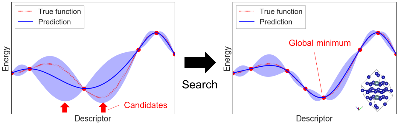
Reference
LAQA
One of the selection-type algorithms.
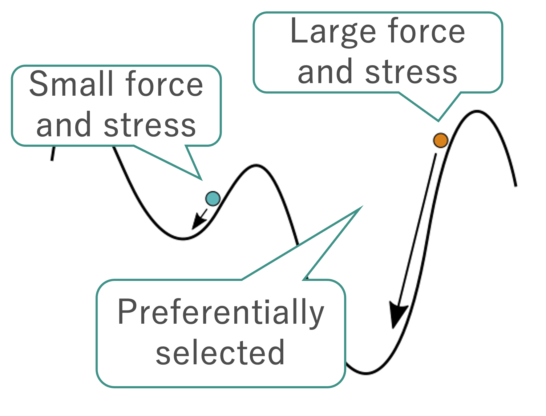
Score $ L $
$$ L = -E + w_F \frac{F^2}{2\Delta F} + w_S S. $$| Symbol | Note |
|---|---|
| $$ E $$ | Energy (eV/atom) |
| $$ w_F $$ | Weight of the force term. Default: $ w_F = 0.1$ |
| $$ F $$ | Averaged norm of the atomic force (eV/Å) |
| $$ \Delta F $$ | Absolute difference of $ F $ from the previous step. $ \Delta F = 1$ for the first step. $ \Delta F = 10^{-6}$ if $ \Delta F \le 10^{-6} $. |
| $$ w_S $$ | Weight of the stress term. Default: $ w_S = 10.0$ |
| $$ S $$ | Average of the absolute values of the components of the stress tensor (eV/Å^3). |