Analysis and Visualization
Last updated: October 16, 2026
Automatic Convex Hull Plotting
In EA-vc simulations of binary and ternary systems, a convex hull plot is automatically generated at the end of each generation by default.
The figure is saved to ./data/convex_hull/conv_hull_gen_{gen}.{fig_fotmat}.
From version 1.5.0, the output interval in generations can be changed with energy_output_interval in the [option] section. The default is 1 (every generation); 0 disables automatic output of the convex-hull plot and hull-distance file. The convex hull and hull distances are still calculated every generation. See Input File > [option] Section for details.
Binary System
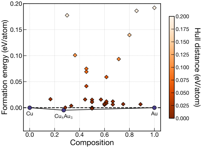
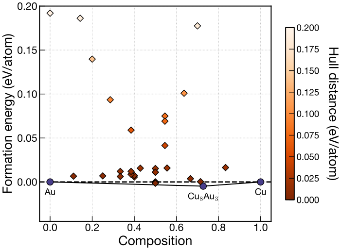
The above figures show examples after the search up to the third generation.
The following input variables can be set in the [visual] section of cryspy.in.
See also CrySPY > Input file > [visual] section.
Here, vmax is the maximum value of the colorbar for the hull distance, and bottom_margin is the margin between the minimum formation energy and the lower limit of the y-axis.
As shown in the left figure, when axis_order = lr (the default setting),
the convex hull plot is drawn so that atype[0] is on the left and atype[1] is on the right.
The right figure shows the case with axis_order = rl.
That is, when atype = Cu Au, the pure Cu crystal is placed on the right side of the plot,
while the pure Au crystal is placed on the left.
Ternary System
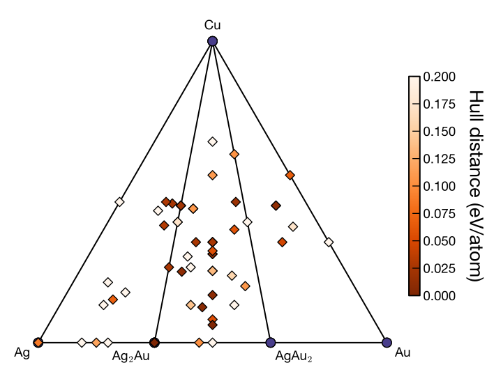
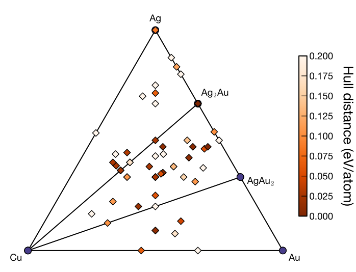
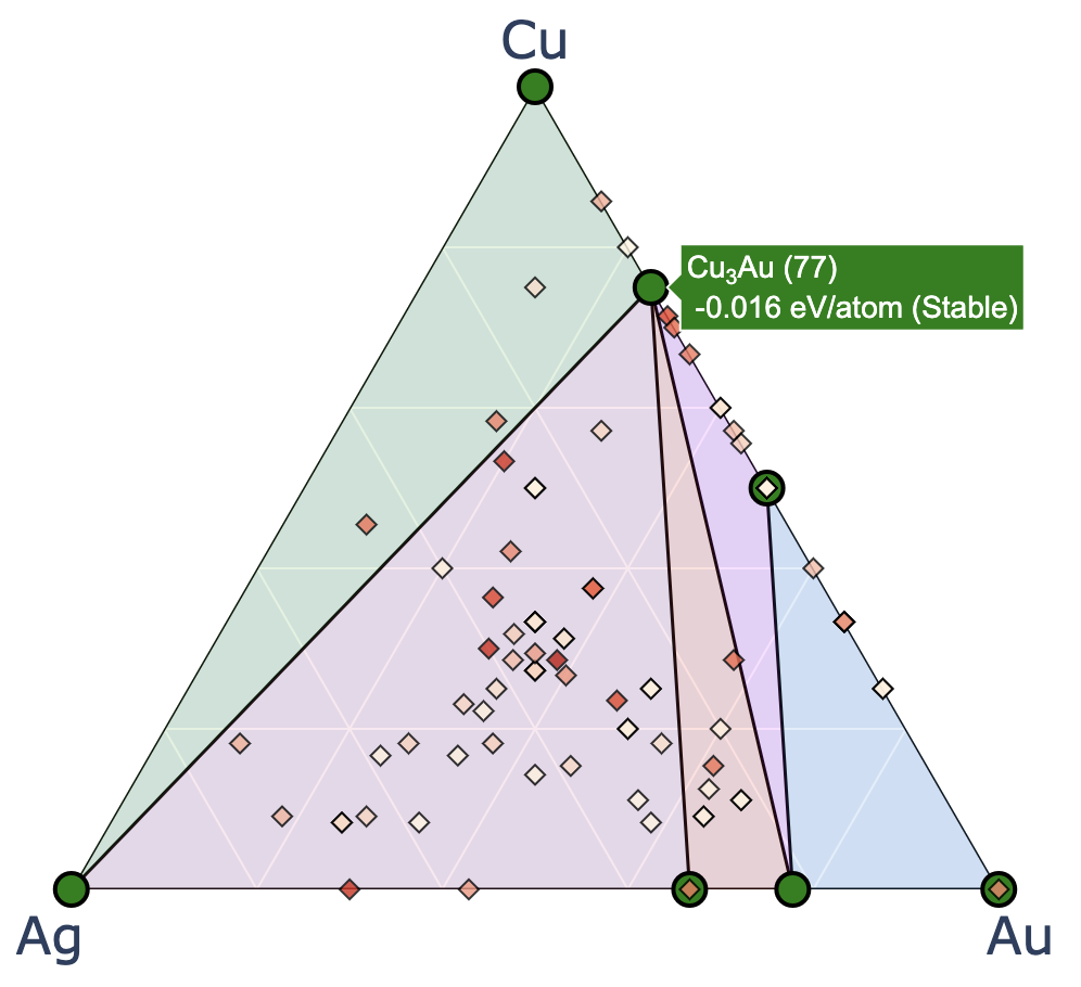
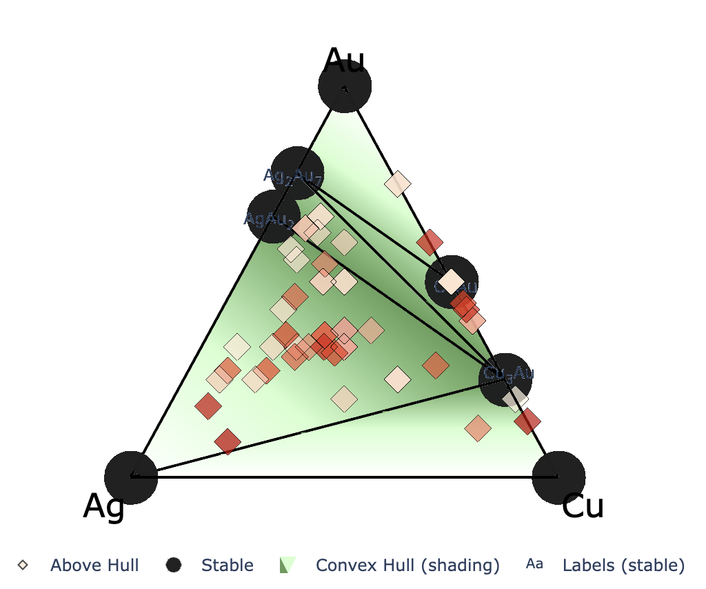
The figures above show the examples for a ternary system.
The following input variables can be set in the [visual] section of cryspy.in.
See also CrySPY > Input file > [visual] section.
Here, show_max specifies the maximum hull distance shown in ternary systems.
In the above example, it is commented out, so the default value None is applied.
When axis_order = tlr (the default setting), atype[0], atype[1], and atype[2] are placed at the top, left, and right vertices, respectively, in the ternary convex hull plot, as shown in the left figure.
Adjust the vertex order accordingly for other permutations such as trl, ltr, etc.
The right figure shows an example with axis_order = ltr.
For atype = Cu Ag Au, Cu is placed at the left vertex, Ag at the top vertex, and Au at the right vertex.
Charge Neutrality Condition
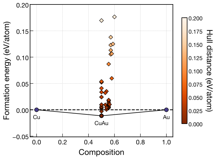
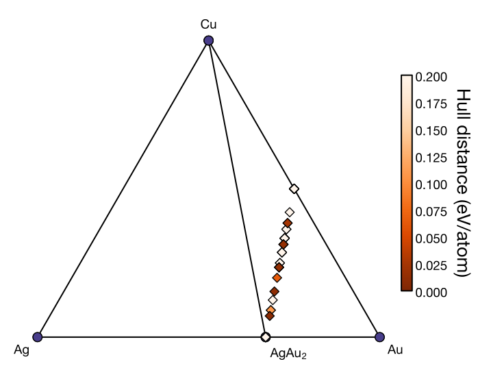
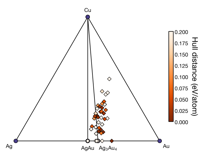
The following convex hull plots show examples with a charge neutrality condition imposed by specifying charge.
See Features > Charge Neutrality Condition for input examples and details on specifying charges.
Binary examples: single-valence (left) and multi-valence (right).
- single-valence:
(Cu, Au) = (+1, -1) - multi-valence:
(Cu, Au) = ((+2, +3), -2)
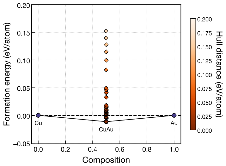
Ternary examples: single-valence (left) and multi-valence (right).
- single-valence:
(Cu, Ag, Au) = (+1, +2, -1) - multi-valence:
(Cu, Ag, Au) = (+1, (+2, +3), -2)
Composition Constraints
From version 1.5.0, min_comp and max_comp can restrict the composition range explored by the search.
When composition constraints are set, the allowed range is shown as a blue region in the convex hull plot.
See Features > Composition Constraints for input examples and an explanation of the plots.
Examples of search results through generation 3 for binary (left) and ternary (right) systems.
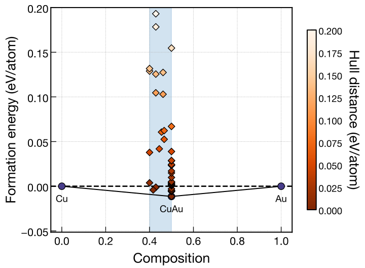
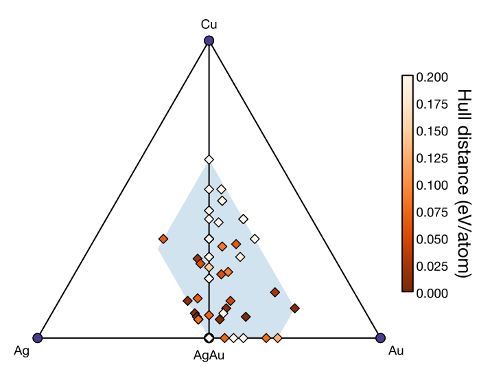
To check the composition range specified in the input without using search results, use the cryspy-Eplot -c option.
Combining Charge Neutrality with Composition Constraints
Composition constraints can also be combined with charge neutrality specified by charge.
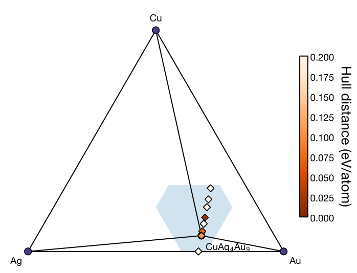
In that case, the blue region represents only the composition constraints, and generated structures must also satisfy charge neutrality within that region.
See Features > Composition Constraints for input examples.
Example of ternary search results through generation 3 with both conditions applied.
Replotting with cryspy-Eplot
If you want to fine-tune the figure and replot it, you can easily do so using the cryspy-Eplot command as follows:
Replotting Specific Generations
When using the cryspy-Eplot command, the following variables can also be specified in the [visual] section in addition to the standard variables above.
plot_min_genplot_max_genref_gen
For example, to replot the figure at generation 2, write the [visual] section as follows:
Then, run the following command:
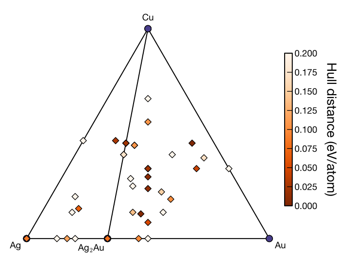
In this case, CrySPY overwrites ./data/convex_hull/conv_hull_gen_{gen}.{fig_fotmat}.
You can specify the range of generations to be plotted using plot_min_gen and plot_max_gen.
When plot_min_gen is set to specify a range (even if its value is 1), the output is saved with a different filename such as ./data/convex_hull/conv_hull_gen_{plot_min_gen}-{plot_max_gen}.{fig_fotmat}, instead of the usual one.
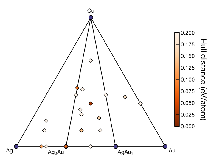
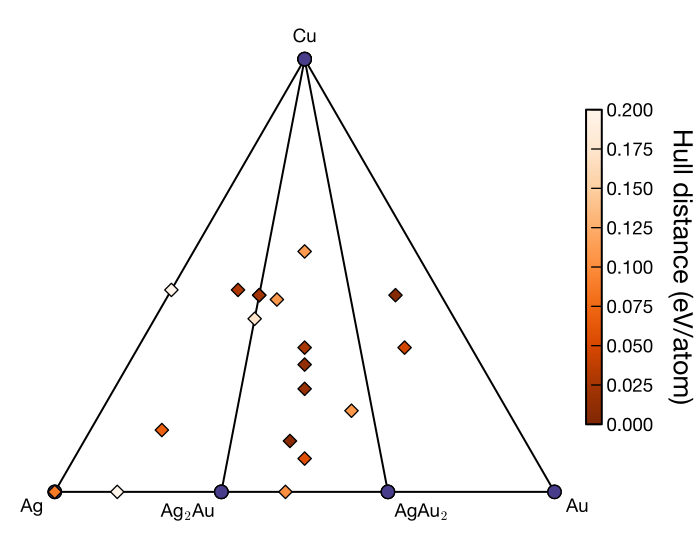
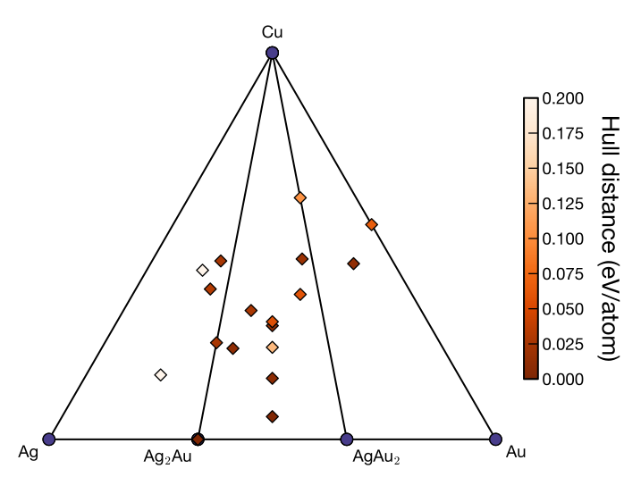
For example, from left to right, the figures above show convex hull plots including only the structures from the first, second, and third generations, respectively.
Note that the convex hull (solid line) in all plots is based on the third generation using ref_gen = 3.
The value of ref_gen must be set to be greater than or equal to plot_max_gen.
As shown in the central figure, to extract only the results of the second generation, specify the following settings in the [visual] section.
If ref_gen is specified, the output filename becomes
conv_hull_gen_{plot_min_gen}-{plot_max_gen}_ref_{ref_gen}.{fig_format}.
Convex Hulls with Compound Terminals
You can also plot a convex hull referenced to compound compositions by specifying terminals in the [visual] section. For an example, see Commands > cryspy-Eplot > Convex Hulls with Compound Terminals.
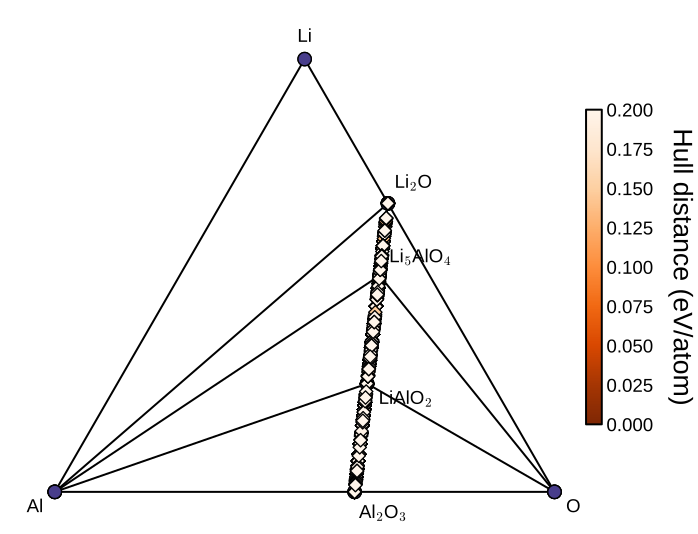
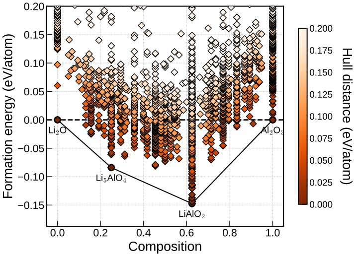
The following example uses Li–Al–O search results through generation 30 with a charge neutrality condition imposed. The left figure shows the ternary convex hull referenced to the elements; the right figure shows the pseudo-binary convex hull referenced to Li2O and Al2O3.
Download Data
It is assumed here that you analyze and visualize CrySPY data on your local PC.
If you use CrySPY on a supercomputer or workstation, download the data to your local machine.
You can delete the work and backup directories if they are not needed, as their file size can be very large.
Jupyter Notebook
Move to the data/ directory in the results you downloaded earlier.
Then, if the CrySPY utility has already been downloaded locally, copy cryspy_analyzer_EA-vc.ipynb.
Alternatively, you can download it directly from GitHub (CrySPY_utility/notebook/).
The Jupyter notebook file includes the same functions as the CrySPY code, allowing you to freely customize the convex hull plots. Execute the cells in order as appropriate, and choosing one of the following options will produce the same plot as the automatic output.
- Binary system, matplotlib
- Ternary system, matplotlib
In the section
- Interactive plot using Plotly,
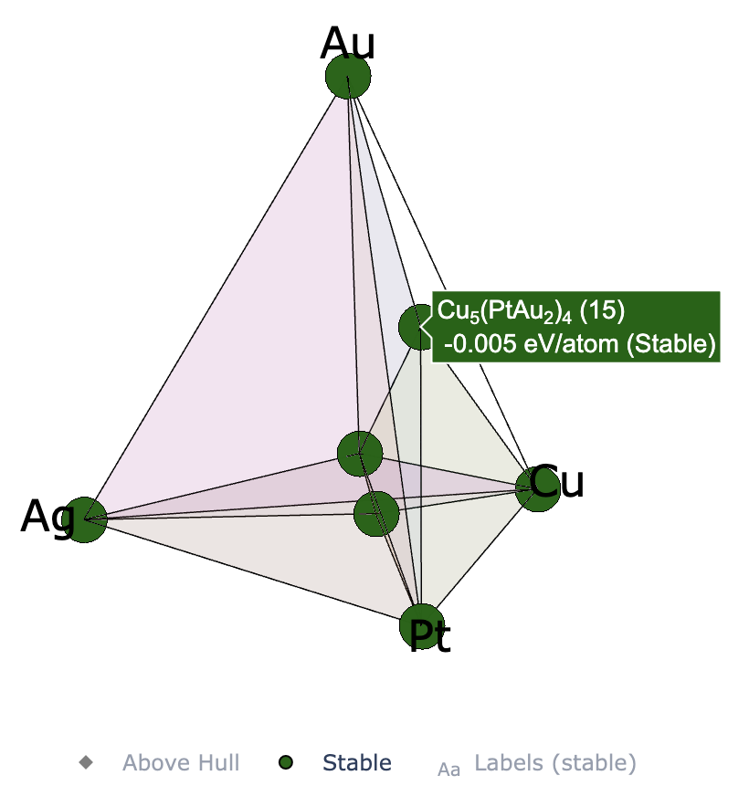
interactive plots using Plotly are available for binary, ternary, and quaternary systems.