Interactive mode (Jupyter Notebook)
2025 March 6
Preparation
When CrySPY is installed, ASE is automatically installed as well. Set up Jupyter to be usable on a workstation or local PC. In this tutorial, Pure Python EMT calculator is used for structure optimization. Note that the accuracy of the EMT potential is poor, as it is intended for demonstration purposes only.
The example notebook also includes code for using the machine learning potential CHGNet. If you want to try CHGNet, make sure to install it in advance using pip.
Input file
Move to your working directory, and copy the example files by one of the following methods.
- Download from CrySPY_utility/examples/interactive
- Copy from CrySPY utility that you installed
Even in interactive mode, cryspy.in is used as the input file.
The calc_in directory is not used in interactive mode.
You can refer to the examples of cryspy.in in the input_examples directory.
Here, the following cryspy.in using EA-vc will be used.
For more details on EA-vc, refer to the EA-vc tutorial.
[basic]
algo = EA-vc
calc_code = ASE
nstage = 1
njob = 10
jobcmd = zsh
jobfile = job_cryspy

[structure]
atype = Cu Au
ll_nat = 0 0
ul_nat = 8 8

[ASE]
ase_python = ase_in.py

[EA]
n_pop = 20
n_crsov = 5
n_perm = 2
n_strain = 2
n_rand = 2
n_add = 3
n_elim = 3
n_subs = 3
target = random
n_elite = 2
n_fittest = 10
slct_func = TNM
t_size = 2
maxgen_ea = 5
end_point = 0.0 0.0

[option]
Notebook
Open cryspy_interactive.ipynb and execute the cells from the top.
Check current working directory
The first cell only checks the files and the contents of cryspy.in.
!pwd
print()
!ls
print()
!cat cryspy.in
Import
Ignore the commented-out sections this time and execute the cell that imports the core libraries for CrySPY’s interactive mode.
# ---------- import
from cryspy.interactive import action
Initialize CrySPY
This cell corresponds to a standard initial run. It reads cryspy.in and generates the initial structures.
# ---------- initial structure generation
action.initialize()
Set calculator
This cell sets the ASE calculator. Here, ASE’s EMT is used.
# ---------- EMT in ASE
from ase.calculators.emt import EMT
calculator = EMT()

# ---------- CHGNet
#from chgnet.model import CHGNetCalculator
#calculator = CHGNetCalculator()
Restart CrySPY
Executing this cell starts the optimization of the previously generated initial structures. In interactive mode, structure optimization calculations are performed sequentially, one by one. A progress bar is also displayed during the process.
# ---------- structure optimization
action.restart(
    njob=20,    # njob=0: njob in cryspy.in will be used
    calculator=calculator,
    optimizer='BFGS',    # 'FIRE', 'BFGS' or 'LBFGS'
    symmetry=True,       # default: True
    fmax=0.01,           # default: 0.01 eV/Å
    steps=2000,          # default: 2000
)
- njob: The number of structures to be optimized in a single execution. If set to 0, the value specified in
cryspy.inis used. - calculator: Assign the previously set calculator.
- optimizer: Select from
FIRE,BFGS, orLBFGS. Specify as a string. - symmetry: If True, structure optimization is performed while preserving symmetry.
- fmax: The maximum atomic force (eV/Å) used for convergence criteria.
- steps: Maximum optimization steps.
If the njob value is set to a small number, execute this cell multiple times to complete the optimization of all initial structures.
When using EA-vc, the following message will be displayed upon completion.
EA is ready
Executing this cell again will trigger generational turnover. Once the next-generation structures are generated, continue executing this cell repeatedly in the same manner.
Show results
Running this cell allows you to display files such as cryspy_rslt_energy_asc.
# ---------- show results
#!cat ./data/cryspy_rslt    # Order of structure optimization completion
!cat ./data/cryspy_rslt_energy_asc    # show energy ascending order
#!sed -n 2,4p ./data/cryspy_rslt    # show i--jth lines
#!tail -n 5 ./data/cryspy_rslt    # show last 5 lines
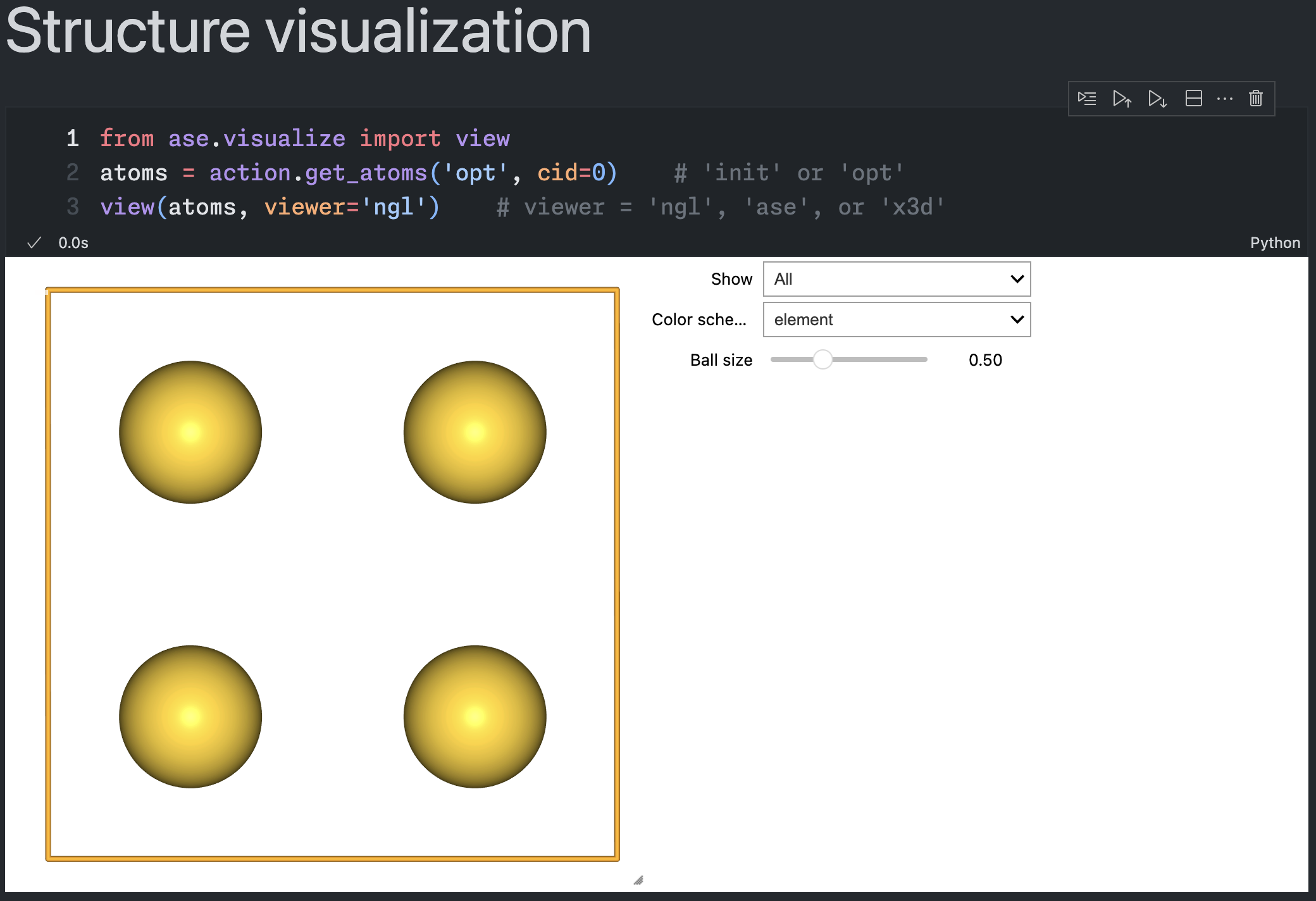
Structure visualization
You can interactively visualize both the initial and optimized structures.
from ase.visualize import view
atoms = action.get_atoms('opt', cid=0)    # 'init' or 'opt'
view(atoms, viewer='ngl')    # viewer = 'ngl', 'ase', or 'x3d'
Changing opt to init in action.get_atoms('opt', cid=0) allows you to check the initial structure.
The cid parameter specifies the structure ID.
Since this utilizes ASE’s functionality, the viewer option supports ngl, ase, and x3d.
To use ngl, you need to install nglview, so make sure to install it via pip in advance.
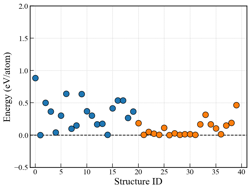
Energy plot for RS, EA
For random search (RS) and evolutionary algorithm (EA), an energy graph shown below can be displayed. In the case of EA-vc, direct energy comparison is not possible due to differences in the number of atoms, so the convex hull plot, discussed later, is used instead.
fig, ax = action.plot_E(
              title=None,
              ymax=2.0,
              ymin=-0.5,
              markersize=12,
              marker_edge_width=1.0,
              marker_edge_color='black',
              alpha=1.0,
          )
Convex hull plot for EA-vc
Interactive plot using Plotly
For EA-vc, an interactive convex hull plot using Plotly is available. When CrySPY is installed, Plotly is automatically installed as well. This convex hull plot utilizes pymatgen’s functionality.
action.interactive_plot_convex_hull(cgen=None, show_unstable=0.2, ternary_style='2d')
- cgen: Which generation’s data to plot up to. If None, data will be plotted up to the latest generation.
- show_unstable: The maximum hull distance value to display on the plot
- ternary_style
- Binary system: ternary_style = ‘2d’
- Ternary system: ternary_style = ‘2d’, ‘3d’
- Quaternary system: ternary_style = ‘3d’
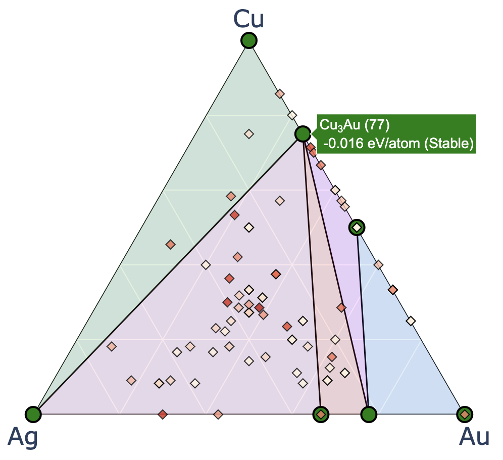
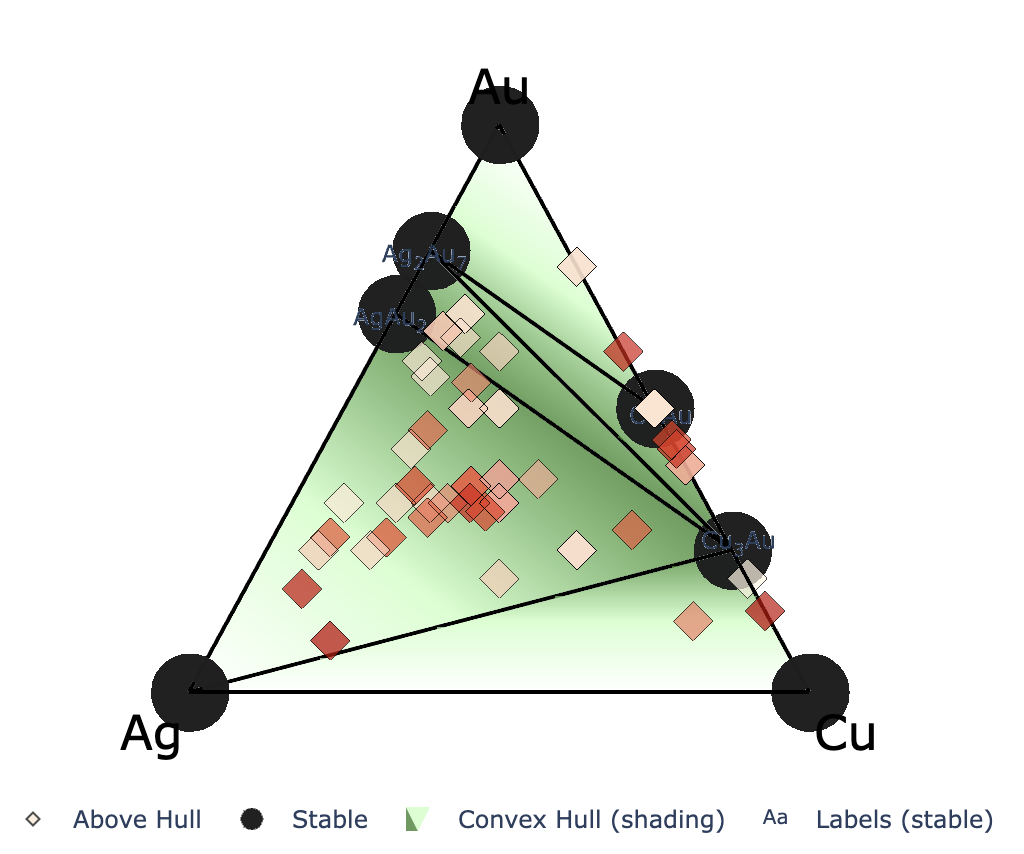
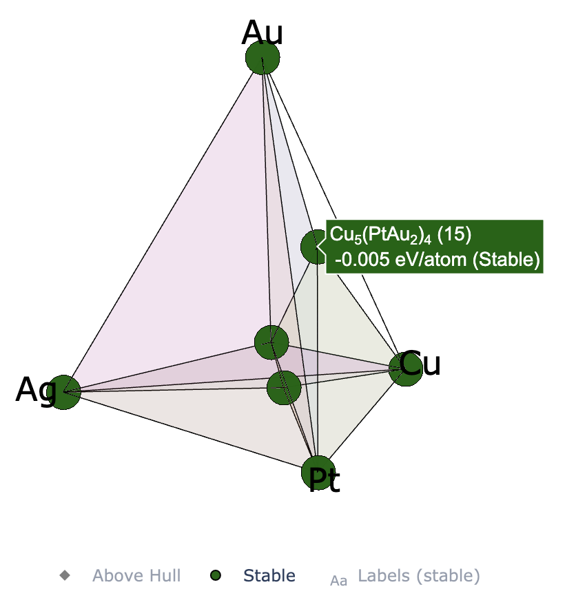
When performing calculations with ternary or quaternary systems instead of binary systems, you can obtain the following interactive plots.
From left to right:
- Ternary system (ternary_style = ‘2d’)
- Ternary system (ternary_style = ‘3d’)
- Quaternary system (ternary_style = ‘3d’)
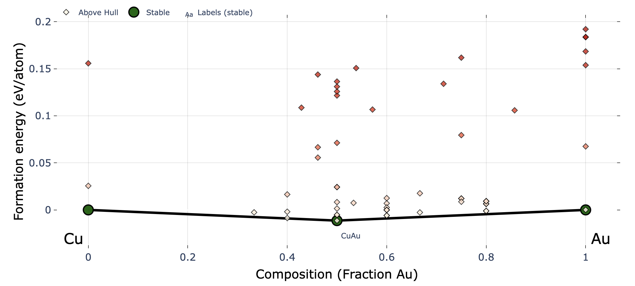
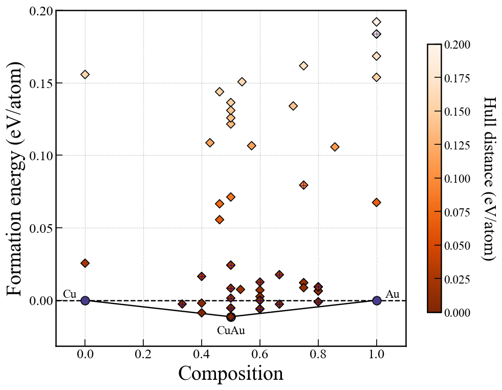
Binary system using matplotlib
Running this cell plots the binary convex hull using matplotlib.
fig, ax = action.plot_convex_hull_binary(
              cgen=None,
              show_max=0.2,
              label_stable=True,
              vmax=0.2,
              bottom_margin=0.02,
          )
fig    # to show plot in jupyter
- cgen: Which generation’s data to plot up to. If None, data will be plotted up to the latest generation.
- show_max: The maximum formation energy to display on the plot
- label_stable: Whether to display the labels (compositions) of stable structures
- vmax: The maximum hull distance in the color bar
- bottom_margin: Bottom margin of y-axis
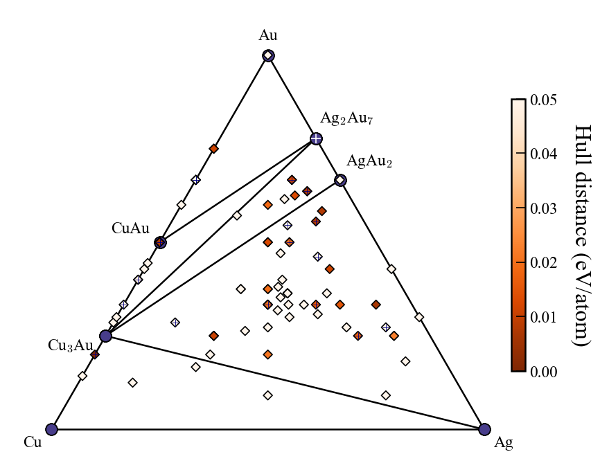
Ternary system using matplotlib
If exploring a ternary system, running this cell will generate a convex hull plot using matplotlib.
fig, ax = action.plot_convex_hull_ternary(
              cgen=None,
              show_max=0.2,
              label_stable=True,
              vmax=0.2,
          )
fig    # to show plot in jupyter
- cgen: Which generation’s data to plot up to. If None, data will be plotted up to the latest generation.
- show_max: The maximum formation energy to display on the plot
- label_stable: Whether to display the labels (compositions) of stable structures
- vmax: The maximum hull distance in the color bar
For example, the following plot can be obtained.